Construction of a Bayesian Network as an Extension of Propositional
Logic
Takuto Enomoto
1
and Masaomi Kimura
2
1
Graduate School of Engineering and Science, Shibaura Institute of Technology,
3-7-5 Toyosu, Koto Ward, Tokyo 135-8548, Japan
2
Department of Information Science and Engineering, Shibaura Institute of Technology,
3-7-5 Toyosu, Koto Ward, Tokyo 135-8548, Japan
Keywords:
Bayesian Network, Association Rule Mining, Propositional Logic.
Abstract:
A Bayesian network is a probabilistic graphical model. Many conventional methods have been proposed for
its construction. However, these methods often result in an incorrect Bayesian network structure. In this
study, to correctly construct a Bayesian network, we extend the concept of propositional logic. We propose
a methodology for constructing a Bayesian network with causal relationships that are extracted only if the
antecedent states are true. In order to determine the logic to be used in constructing the Bayesian network, we
propose the use of association rule mining such as the Apriori algorithm. We evaluate the proposed method
by comparing its result with that of traditional method, such as Bayesian Dirichlet equivalent uniform (BDeu)
score evaluation with a hill climbing algorithm, that shows that our method generates a network with more
necessary arcs than that generated by the traditional method.
1 INTRODUCTION
A Bayesian network is a probabilistic graphical model
that represents the causal relationships between ran-
dom variables as a directed acyclic graph (Pearl,
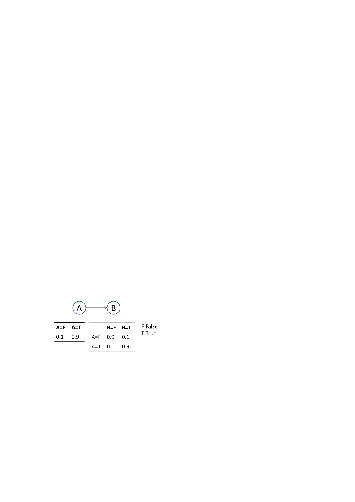
1985). Figure 1 shows an example of a Bayesian net-
work model.
Figure 1: Example of a Bayesian network model.
In Fig. 1, circles having a character denote ran-
dom variables. Causal relationships between these
random variables are represented by arcs; the tip of
the arc points represents a resulting event (conse-
quent), and the end of the arc points represents a
causal event (antecedent). The tables in Fig. 1 are
called conditional probability tables (CPTs) and show
the conditional probabilities of a consequent (B) given
an antecedent (A).
Many methods have been proposed for con-
structing Bayesian networks. They optimize an
evaluation function based on a marginal likeli-
hood function, such as Bayesian information crite-
rion (Schwarz, 1978), Akaike’s information crite-
rion (Akaike, 1973), K2 score (Cooper and Her-
skovits, 1992) and Bayesian Dirichlet equivalent uni-
form (BDeu) (Hecerman and Chickering, 1995). In
addition, they search for an optimal value in their
function using a heuristic algorithm, such as a greedy
algorithm (Cormen et al., 2009), a genetic algorithm
(Holland, 1992),(S. Fukuda and T.Yoshihiro, 2014)
and a hill climbing algorithm (I. Tsmardinos and Alif-
eris, 2006),(J. A. Gamez and Puerta, 2015). However,
we presume that they often incorrectly identified the
Bayesian network structures.
In this study, to correctly construct a Bayesian net-
work, we employ the concept of propositional logic.
A propositional logic can handle a statement that is
represented as true or false. In propositional logic, a
logical expression is represented as a statement, e.g.,
gif A, then B,h because A and B both deal with causal
structures.
The Venn diagrams shown in Fig. 2 illustrate a
causal relationship between an antecedent (A) and a
consequent (B) expressed in a CPT of a Bayesian net-
Enomoto, T. and Kimura, M..
Construction of a Bayesian Network as an Extension of Propositional Logic.
In Proceedings of the 7th International Joint Conference on Knowledge Discovery, Knowledge Engineering and Knowledge Management (IC3K 2015) - Volume 1: KDIR, pages 211-217
ISBN: 978-989-758-158-8
Copyright
c
2015 by SCITEPRESS – Science and Technology Publications, Lda. All rights reserved
211

work (on the left) and an implicational relation rule of
propositional logic (A → B) (on the right).
Figure 2: Venn diagram on the left illustrates a causal re-
lationship according to a Bayesian network, and the one on
the right illustrates an implicational relation rule of propo-
sitional logic.
In a propositional logic, whether or not a causal
relationship holds is expressed in binary. On the other
hand,in a Bayesian network, the existence of a causal
relationship is not necessarily represented in binary
but instead by a probability. Figure 2 illustrates these
situations with Venn diagrams to clarify their differ-
ences. Realistically, whether or not a causal relation-
ship is established cannot be treated in binary as done
in propositional logic because there is no guarantee
that the causal relation infallibly holds true for any
case in an actual setting. In fact, in a case where the
probability of the occurrence of an event is extremely
high, we consider that the causal relationship holds
true. Therefore, we regard a Bayesian network as an
extension of propositional logic.
If we limit ourselves to a one-to-one relation be-
tween an antecedent and a consequent, as in Fig. 1,
the combinations of values that A and B can be are as
follows:
A is T ⇒ B is T
A is T ⇒ B is F
A is F ⇒ B is T
A is F ⇒ B is F
The traditional methods for constructing a
Bayesian network optimized all the combinations of
causal relationships. However, in the implication re-
lationship of propositional logic, if an antecedent is
true, a causal relationship can either be true or false,
and if an antecedent is false, the causal relationship
is true. In other words, when an antecedent is false,
a consequent has nothing to do with the establish-
ment of a causal relationship. Therefore, we regard
a Bayesian network as an extension of propositional
logic, and causal relationships with a false antecedent
state need not be taken into account when construct-
ing a Bayesian network.
Therefore, we have proposed a methodology for
constructing a Bayesian network whose causal rela-
tionships are removed if the antecedent state is false
using association rule mining.
2 METHODS
In order to construct a Bayesian network as an ex-
tension of propositional logic, we need to determine
the existence or non-existence of causal relationships
in all random variables. In addition, we must extract
only the causal relationships whose antecedent is T .
Therefore, we can effectively extract causal relation-
ship candidates using association rule mining.
Association rule mining is a typical method
for identifying relationships between variables in
large-scale transactional data (Piatetsky and Frawley,
1991), (R. Agrawal and Swami, 1993). This method
uses three indices called support, confidence, and
lift to evaluate a causal relationship, as illustrated in
Equations (1), (2) and (3) below. Let P(A) denote a
marginal probability of a random variable A, then
support(A ⇒ B) = P(A, B), (1)
confidence(A ⇒ B) = P(B|A), (2)
lift(A ⇒ B) =
P(A, B)
P(A)P(B)
. (3)
Equation 1 expresses the co-occurrence frequency be-
tween random variables and is defined as a percentage
of the transactions that contain both an antecedent and
a consequent in all data transactions. Equation 2 is a
conditional probability and is defined as a percentage
of the transactions that contain both an antecedent and
a consequent in all data transactions that include the
antecedent. Equation 3 is a measurement of the in-
terdependence between the random variables. If its
value is higher than 1.0, the antecedent and conse-
quent are regarded as having a dependency.
Apriori is a classic algorithm for use in associ-
ation rule mining. In order to extract candidates of
random variable combinations that have a correlation,
this algorithm focuses only on combinations of ran-
dom variables that frequently appear in a data store.
The Apriori algorithm is applied when either a ran-
dom variable or combination of random variables oc-
cur infrequently.
2.1 Bayesian Network and CPT
Relationships
Since the values in CPTs are probabilities, they range
from 0 to 1. However, the value assignments in
CPTs cannot be independent from the structure of the
KDIR 2015 - 7th International Conference on Knowledge Discovery and Information Retrieval
212

Bayesian network. Figure 3 demonstrates a situation
that is an example of a contradictory Bayesian net-
work model where the diagram assumes a causal rela-
tionship between A and B, although its CPT indicates
no causal relationship between them.
Figure 3: Bayesian network model that cannot predict a
consequent if an antecedent is T .
This Bayesian network model has an arc from A
to B. However, the probabilities of any combination
of values of random variable A and random variable
B are identical; namely, when A is true, the value of
random variable B cannot be predicted to be true or
false.
Moreover, Fig. 4 indicates no causal relationship
between A and B. For all values of random variable
A, the value of random variable B is true with a prob-
ability of 0.8. As such, A and B are independent,
P(B|A) = P(B).
Figure 4: Bayesian network model that shows no causal re-
lationship.
In order to exclude these types of contradictory
networks, our method targets networks whose proba-
bilities in the CPTs are less than θ
l
or more than θ
m
when the antecedent is T , as in Fig. 5, where the val-
ues of θ
l
and θ
m
are 0.2 and 0.8, respectively.
2.2 Causal Relationship Extraction
using Confidence Values
Association rule mining can efficiently extract causal
relationship candidates whose support values are fre-
quently high using the Apriori algorithm. In other
words, even if random variables have strong asso-
ciations, a candidate is not extracted when its sup-
port value is low. To extract these causal relation-
Figure 5: Bayesian network examples containing causal re-
lationships. When an antecedent is T , the consequent is
F(a), and when all random variables in an antecedent are T ,
the consequent is T(b).
ship candidates, we focus on the use of confidence
values in the Apriori algorithm. Confidence measures
the association strength for a random variable combi-
nation. Even though the Apriori algorithm only ex-
tracts causal relationship candidates possessing high
support values, in our study, we must extract causal
relationships possessing strong associations. There-
fore, we extract the random variable combination that
is a causal relationship candidate if its confidence
and support exceeds certain threshold values. In this
study, we use a high threshold for confidence and a
low threshold for support to efficiently extract causal
relationship candidates.
2.3 Extraction of Causal Relationship
with Low Consequent Probability
In this study, causal relationships whose antecedent is
T , namely {An antecedent is T ⇒ A consequent is T}
and {An antecedent is T ⇒ A consequent is F}, are
taken into account. However, the Apriori algorithm
only extracts causal relationship candidates whose
antecedents and consequents are frequently T , i.e.,
causal relationships whose consequents are frequently
F are not extracted. In order to extract these candi-
dates, if the causal relationships are not extracted by
the Apriori algorithm, the random variable of the con-
sequent in the CPT is swapped for its complement.
Figure 6 illustrates this method using the Bayesian
network.
In this Bayesian network, imagine that {B ⇒ A}
is not extracted by the Apriori algorithm because the
consequent of the causal relationship is frequently F.
Therefore, in order to extract it, we convert the con-
sequent A to its complement A
c
. Figure 7 shows this
Construction of a Bayesian Network as an Extension of Propositional Logic
213

Figure 6: A Bayesian network for explaining our proposed
method.
Figure 7: Swapping of probabilities in the CPT values.
conversion.
The Bayesian network and table on the right in
Fig. 7 are obtained after the conversion that enables
the Apriori algorithm to extract this causal relation-
ship if the support is greater than the given threshold
value.
2.4 Extraction of Causal Relationships
with Plural Random Variables in
Antecedents
When causal relationships have plural random vari-
ables in their antecedents, it is possible that they may
not be extracted even if there is a strong association.
For example, {D, E ⇒ C} in Fig. 6 is not extracted
because random variable C tends to be T only when
both random variable D and E are T . In other words,
when one of the random variables is not T , C is hardly
ever T. Therefore, the confidence values of { D ⇒ C}
and {E ⇒ C} are low. In such a case, when the Apri-
ori algorithm is executed, these causal relationships
are eliminated during the process. Because of this,
{D, E ⇒ C} is not extracted even if its confidence
value exceeds the threshold.
In order to extract such candidates, if the confi-
dence value of a causal relationship is lower than the
given threshold, we compare it with the confidence
value of the causal relationship that then adds an op-
tional random variable to the antecedent. If the latter
value is higher than the original, it is not eliminated
until the next iteration of the Apriori algorithm. In
the case of Fig. 7, this allows us to keep { D ⇒ C}
and {E ⇒ C} until {D, E ⇒ C} is extracted.
2.5 Selecting and Linking for Causal
Relationship Candidates
With our method, a Bayesian network is obtained by
combining the causal relationship candidates.
Keep in mind that each random variable in a
Bayesian network appears only once as a consequent
variable. Based on this fact, we combine causal re-
lationships with the highest lift from candidates that
share the same consequent. For example, assume that
the following causal relationship candidates are found
for the Bayesian network in Fig. 6, which are sorted
in descending order of lift.
1.
D, E ⇒ C
2.
B ⇒ C
3.
B ⇒ A
4.
A, C ⇒ B
In this case, first,
D, E ⇒ C
is integrated in a
Bayesian network. Second, whether or not
B ⇒ C
is taken account. Since the causal relationship pos-
sessing random variable C in the consequent has al-
ready been integrated, it is not employed. Then
B ⇒
A
and
A, C ⇒ B
are integrated. Figure 8 shows a
Bayesian network constructed from these causal rela-
tionship candidates.
Figure 8: Bayesian network constructed from causal rela-
tionships candidates.
2.6 Direction Determination for
Dual-directional Causal
Relationship
When causal relationships are integrated, dual-
directional causalities can be created, as shown in Fig.
8. If we find such causalities, we must establish the
correct direction by comparing the products of the
KDIR 2015 - 7th International Conference on Knowledge Discovery and Information Retrieval
214

causal relationship confidence values. With respect
to the dual-directional causalities in the Bayesian net-
work in Fig. 8, the equations to be compared are
P(B|C)P(B|A) and P(B|A, C).
3 EXPERIMENT
In order to evaluate the proposed method, we com-
pared the Bayesian network created by the proposed
method with one created by the BDeu score evalua-
tion with a hill climbing algorithm(J. A. Gamez and
Puerta, 2015). We created sampling data from an
original Bayesian network as shown in Fig. 9, where
the values of θ
l
and θ
m
are 0.2 and 0.8, respectively.
Figure 9: Bayesian network for our experiment.
The parameters of association rule mining in the
proposed method were as follows:
• The support threshold = 0.01 (s
1
), 0.015 (s
2
), 0.02
(s
3
),
• The confidence threshold = 0.7.
In this experiment, we used three support values.
Confidence value was fixed to be 0.7, because exper-
imental results did not change, while it was changed
to 0.6, 0.65, 0.7 and 0.75.
After constructing the Bayesian networks, we
used Hamming distance in the original Bayesian net-
work to compare the constructed Bayesian networks.
The Hamming distance counts the difference between
the two off-diagonal matrices representing directed
graphs. The Hamming distance of exactly the same
graph is zero. The more different the graphs are,
the greater the value of the Hamming distance is.
Therefore, if the Hamming distance for the proposed
method is shorter than that for BDeu with a hill
climbing algorithm (hereafter, we simply call BDeu),
we can say that our method can give more accurate
Bayesian network than BDeu.
3.1 Results and Discussions
Figure 10 shows the results obtained using BDeu, and
Fig. 11, 12 and 13 show the results obtained by the
proposed method. Table 1 shows the numbers of the
arcs and Hamming distances.
Figure 10: A Bayesian network constructed by BDeu with
a hill climbing algorithm.
Figure 11: A Bayesian network constructed by our pro-
posed method with the support threshold s
1
.
Table 1: The numbers of arcs and Hamming distance.
BDeu s
1
s
2
s
3
Total number of arcs 14 16 13 9
Total number of correct arcs 10 10 10 3
Hamming distance 8 10 7 17
In the Bayesian network constructed by BDeu,
mainly inverted forks, such as
C, D ⇒ E
and
J, K, L ⇒ M
were not reproduced. This is because
Construction of a Bayesian Network as an Extension of Propositional Logic
215

Figure 12: A Bayesian network constructed by our pro-
posed method with the support threshold s
2
.
Figure 13: A Bayesian network constructed by our pro-
posed method with the support threshold s
3
.
the number of random variables in an antecedent was
too many to be optimized. In the proposed method, s
2
had most shortest Hamming distance of all. In addi-
tion, this method reproduced all inverted forks. In the
case that the support value was 0.01, the Bayesian net-
work had causal relationship that did not exist in the
original one, such as
A, D, L ⇒ J
. This is because
a rule whose antecedent had many random variables
tended to have low suppprt value and high confidence
value. On the other hand, in the case of support value
was 0.02, inverted forks such as
C, D ⇒ E
and
J, K, L ⇒ M
were not reproduced because of the
same reason for the case with the low support value,
0.01.
Even in the case with the support value s
2
, there
were some causal relationships that could not be re-
produced. We explain its reason with the relationships
as follows:
•
B ⇒ A
,
•
I ⇒ K
.
The causal relationship
B ⇒ A
had antecedent
and consequent opposite to
A ⇒ B
in the original
Bayesian network. Both
A ⇒ B
and
B ⇒ A
were
extracted by our Apriori algorithm. However, since
P(A|B) was higher than P(B|A), the causal relation-
ship
B ⇒ A
was adapted in our method. The rea-
son why P(A|B) was higher was that P(A) was higher
than P(B). Remembering that we generated data of B
from the value of A following the probability P(B|A)
and P(B|A
c
) in our simulation, this can occur if both
P(B|A) and P(B|A
c
) are reasonably low. In practice,
we might draw an arc from B to A if we manually
build the network, if P(A|B) is higher than P(B|A). It
can be said that our method simulated such cases.
The causal relationship
I ⇒ K
was extracted in
Apriori algorithm. However, the lift value of
H ⇒
K
is higher than that of
I ⇒ J
. Therefore,
I ⇒
K
was not integrated.
We can see that the Hamming distance is longer
in the network generated by BDeu than that in the s
2
.
However, Hamming distance of s
1
and s
3
are longer
than it. Therefore, our proposed method is effec-
tive for creating a Bayesian network when appropriate
support and confidence value are determined.
4 CONCLUSION AND FUTURE
WORKS
Many conventional methods have been proposed for
constructing Bayesian networks that optimize com-
binations of the occurrences of causal relationships.
However, they often yield an incorrect Bayesian net-
work structure.
If we correspond the establishment of a causal re-
lationship in a Bayesian network to a probability with
the value 0.0 or 1.0, we can regard the Bayesian net-
work as a combination of propositional logic state-
ments. In this study, based on this concept, we pro-
posed a method to construct a Bayesian network as an
extension of propositional logic to determine a correct
Bayesian network structure.
The proposed construction method uses associa-
tion rule mining. We extracted causal relationship
candidates using the confidence values in the Apriori
algorithm. We have also proposed a method for ex-
tracting causal relationships whose antecedents have
plural random variables and consequents are less fre-
quently T . Finally, we linked the obtained causal re-
lationship to obtain a Bayesian network.
We compared the resultant Bayesian network con-
structed using our method with those constructed us-
KDIR 2015 - 7th International Conference on Knowledge Discovery and Information Retrieval
216
ing BDeu score evaluations. We found that, when ap-
propriate support and confidence value are used, our
proposed method is effective to create a Bayesian net-
work.
In future studies, we will discuss improvements to
calculate appropriate values of thresholds for support
and confidence. We need to confirm the limit of θ
l
and θ
m
that we can apply this method. In addition, we
will discuss the extension of our approach to multiple-
valued logic.
REFERENCES
Akaike, H. (1973). Information theory and an extension
of the maximum likelihood princi- ple. Proceedings
of the 2nd International Symposium on Information
Theory, pages 267–281.
Cooper, G. and Herskovits, E. (1992). A bayesian method
for the induction of probabilistic networks from data,
machine learning. Machine Learning, 9:309–347.
Cormen, T., Leiserson, C., and Rivest, R. (2009). Introduc-
tion to Algorithms, 3rd Edition. MIT.
Hecerman, D. and Chickering, D. (1995). Learning
bayesian networks: The combination of knowledge
and statistical data. The combination of knowledge
and statistical data, 20:197–243.
Holland, J. H. (1992). Adaptation in natural and artificial
systems: An introductory analysis with applications to
biology, control, and artificial intelligence. MIT.
I. Tsmardinos, L. E. B. and Aliferis, C. F. (2006). The max-
min hill-climbing bayesian network bayesian network
structure learning algorithm. Machine Learning, 65.
J. A. Gamez, J. L. M. and Puerta, J. M. (2015). Struc-
tural learning of bayesian networks via constrained
hill climbing algorithms: Adjusting trade-off between
efficiency and accuracy. International Journal of In-
telligent Systems, 30.
Pearl, J. (1985). Bayesian networks: A model of self-
activated memory for evidential reasoning. Proceed-
ings of the 7th Conference of the Cognitive Science
Society, pages 329–334.
Piatetsky, G. and Frawley, W. J. (1991). Know ledge Dis-
covery in Databases. MIT.
R. Agrawal, T. I. and Swami, A. (1993). Mining association
rules between sets of items in large databases. , In
Proceedings of the 1993 ACM SIGMOD International
Conference on Management of Data, pages 207–216.
S. Fukuda, Y. Y. and T.Yoshihiro (2014). A probability-
based evolutionary algorithm with mutations to learn
bayesian networks. International Journal of Artificial
Intelligence and Interactive Multimedia, 3:7–13.
Schwarz, G. (1978). Estimating the dimension of a model.
The Annals of Statistics, 6:461–464.
Construction of a Bayesian Network as an Extension of Propositional Logic
217
