Application of Adaptive Differential Evolution for Model Identiﬁcation in

Furnace Optimized Control System

Miguel Leon

, Magnus Evestedt

and Ning Xiong

Innovation, Design and Tecnology Department, Malardalen University, Vasteras, Sweden

Industrial Systems, Prevas, Vasteras, Sweden

Keywords:

Differential Evolution, Optimization, Model Identiﬁcation, Temperature Estimation.

Abstract:

Accurate system modelling is an important prerequisite for optimized process control in modern industrial

scenarios. The task of parameter identiﬁcation for a model can be considered as an optimization problem

of searching for a set of continuous parameters to minimize the discrepancy between the model outputs and

true output values. Differential Evolution (DE), as a class of population-based and global search algorithms,

has strong potential to be employed here to solve this problem. Nevertheless, the performance of DE is

rather sensitive to its two running parameters: scaling factor and crossover rate. Improper setting of these

two parameters may cause weak performance of DE in real applications. This paper presents a new adaptive

algorithm for DE, which does not require good parameter values to be speciﬁed by users in advance. Our

new algorithm is established by integration of greedy search into the original DE algorithm. Greedy search

is conducted repeatedly during the running of DE to reach better parameter assignments in the neighborhood.

We have applied our adaptive DE algorithm for process model identiﬁcation in a Furnace Optimized Control

System (FOCS). The experiment results revealed that our adaptive DE algorithm yielded process models

that estimated temperatures inside a furnace more precisely than those produced by using the original DE

algorithm.

1 INTRODUCTION

System modelling and identiﬁcation provide an im-

portant basis for optimized process control in modern

industrial scenarios. Its main goal is to identify a pro-

cess model that is able to accurately predict the output

of a system in response to a set of inputs. Generally,

a process model can be constructed in two steps. In

the ﬁrst step, the structure of the model is determined

in terms of expert knowledge and insight into the pro-

cess. In the second step, the parameters of the struc-

tured model are to be identiﬁed. This can be consid-

ered as an optimization problem of searching for a set

of continuous parameters to minimize the discrepancy

between the model outputs and true output values on

a set of training samples.

Traditionally, the methods such as Least Mean

Square (LMS) algorithm or Recursive Least Square

Estimation (RLS) algorithms have been used to solve

the model parameter identiﬁcation problems. How-

ever, they are subject to two limitations. First, they

were developed for linear system identiﬁcation, i.e.

when the process model is assumed to be linear. Sec-

ond, they are essentially derivative-based optimiza-

tion techniques and may fail to ﬁnd the optimal solu-

tion when locating many (model) parameters in high

dimensional spaces.

This paper advocates the application of Differ-

ential Evolution (DE) (Storn and Price, 1997) algo-

rithms to solve the parameter identiﬁcation problems

for nonlinear process models. DE presents a class

of evolutionary computing techniques that perform

population-based and beam search, thereby exhibit-

ing strong global search ability in complex, non-linear

and high dimensional spaces (Xiong et al., 2015). DE

differs from many other evolutionary algorithms in

that mutation in DE is based on differences of pair(s)

of individuals randomly selected. Thus, the direction

and magnitude of the search is decided by the distri-

bution of solutions instead of a pre-speciﬁed probabil-

ity density function. The merits of DE include simple

and compact structure, easy use, as well as high con-

vergence speed, which make it quite competitive in

comparison with other evolutionary algorithms.

However, in real applications, the performance of

DE is largely dependent on the values of scaling factor

Leon, M., Evestedt, M. and Xiong, N..

Application of Adaptive Differential Evolution for Model Identiﬁcation in Furnace Optimized Control System.

In Proceedings of the 7th International Joint Conference on Computational Intelligence (IJCCI 2015) - Volume 1: ECTA, pages 48-54

ISBN: 978-989-758-157-1

and crossover rate, which are two important control

parameters of DE. Improper setting of such parame-

ters will lead to low quality of solutions found by DE.

Yet ﬁnding suitable values for them is by no means a

trivial task, it involves a trial-and-error procedure that

is time consuming.

In this paper we present a new adaptive algorithm

for DE, which does not require good parameter val-

ues (scaling factor and crossover rate) to be speciﬁed

by users beforehand. Our new algorithm is estab-

lished by integration of greedy search into the original

DE algorithm. Greedy search is conducted repeatedly

during the running of DE to reach better parameter

assignments in the neighborhood. So far we have ap-

plied our adaptive DE algorithm for process model

identiﬁcation in a Furnace Optimized Control System

(FOCS). The experiment results revealed that our al-

gorithm yielded process models that estimated tem-

peratures inside a furnace more precisely than those

produced by using the original DE algorithm.

The remainder of the paper is organized as fol-

lows. Section 2 brieﬂy describes the application sce-

nario. The original DE algorithm is outlined in Sec-

tion 3, which is followed by the new adaptive DE al-

gorithm in Section 4. Section 5 presents the results

of experiments for model identiﬁcation in a Furnace

Optimized Control System. Section 6 discusses some

relevant works. Finally, concluding remarks are given

in Section 7.

2 PROBLEM FORMULATION

Energy consumption and environmental considera-

tion are important issues to be handled within the

steel industry today. In this respect, inventing and

developing new ways to decrease fuel and emission

levels in steel production and treating are crucial to

production economy. The FOCS system was devel-

oped for reheating furnaces in the early 1980s, and

has since grown to be the most commonly used sys-

tem in the Scandinavian steel industry, (Norberg and

Leden, 1988).

Due to the harsh environment inside the reheating

furnace, the temperature of the heated steel cannot be

measured continuously. Therefore, the FOCS system

core is a temperature calculation model that utilizes

temperature sensor measurements in the walls inside

the furnace as well as current fuel ﬂow, to estimate the

temperature in the heated material. In order to gain

optimal control performance, it is crucial to estimate

the temperatures accurately.

The temperature inside the material can be mea-

sured through the furnace by a test measurement

setup. This is normally done 2-3 times every year to

certify the furnace operation. The measurements are

also used to calibrate the FOCS temperature calcula-

tion model, by changing the model parameters to ﬁt

the model output to the measurements. The calibra-

tion is performed manually and can be a tedious task

due to many parameters and evaluation of several test

measurements simultaneously.

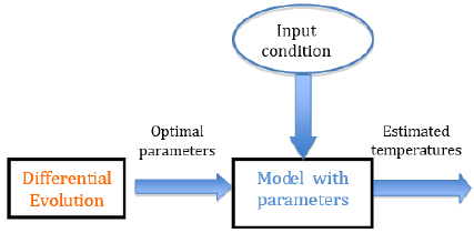
We attempted to apply DE algorithms to facilitate

the automatic determination of the parameters of this

process model. The goal is to ﬁnd such a set of pa-

rameters to minimize the error between the estimated

temperatures from the model and the actual tempera-

tures obtained from the measurements. After the ex-

ecution of DE, we acquire the optimal parameters of

the model, as shown in Fig.1. Subsequently this op-

timal model can be employed in future occasions to

produce reliable estimates of temperatures based on

input conditions.

Figure 1: DE, parameterized model, and temperature esti-

mation.

3 DIFFERENTIAL EVOLUTION

The DE algorithm proposed by R. Storn and K. Price

in 1997 (Storn and Price, 1997) is an stochastic and

population based evolutionary algorithm for global

numerical optimization. The population is compose

by N

individuals, solutions of the problem, repre-

sented by X

i,G

= {x

i,1

, x

i,2

, . . . , x

i,D

}, where i =1, 2,. . . ,

and represents the ith individual, D is the dimen-

sion of the problem and G stands for the generation

that the population belong. DE has three main op-

erators at every generation G: mutation, crossover

and selection. The notation used to name them is

DE/x/y/z, where x represents the mutation strategy

used, y is the number of difference of individuals used

in the mutation strategy and z stands for the crossover

method used. Next we shall brieﬂy describe these

three operators used in a basic DE algorithm.

Mutation: In this ﬁrst step, NP mutant vectors are

created using individuals randomly selected from the

current population. Indeed there are a lot of mutation

Application of Adaptive Differential Evolution for Model Identiﬁcation in Furnace Optimized Control System

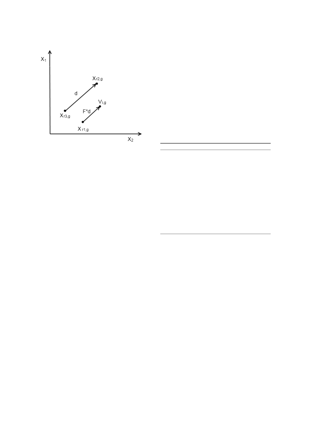
Figure 2: Random mutation with one difference vector.

strategies which can be used to generate mutant vec-

tors. But only the random mutation strategy will be

explained below. The other mutation strategies and

their performance are discussed in (Leon and Xiong,

2014a). The calculation of the mutant vector V

i,G

us-

ing the random mutation strategy is given in Eq.1.1.

i,G

= X

+ F × (X

− X

) (1)

where r

, r

; r

are random integers from 1 to N

, and

F is the scaling factor inside the interval [0, 2]. Fig.

2 shows how this mutation strategy works, where d is

the difference vector between X

and X

As can be seen from Eq. 1,, values in the mutant

vector V

i,G

may violate pre-deﬁned boundary con-

straints for the decision variables. To repair such ille-

gal solution (if it emerges), we modify V

i,G

according

to Eq.2.

i,G

[ j] =

(

(Low[ j] if V

i,G

[ j] < Low[ j],

(U pper[ j] if V

i,G

[ j] > U pper[ j].

(2)

where V

i,G

[ j] denotes the jth component of vector

i,G

, and Low[j] and Upper[j] stand for the low and

upper bounds of the jth decision variable respectively.

Crossover: In this second step, the parent solution

i,G

from the current population and the mutant vector

i,G

are recombined to create a new solution. This

new solution is called trial vector and it is represented

by T

i,G

. Every parameter inside the trial vector is

generated according Eq. 3. This equation ensures that

i,G

is different from X

i,G

in one component at least.

i,G

[ j] =

(

i,G

[ j] if rand[0, 1] <= CR or j = j

rand

i,G

[ j] otherwise

(3)

where j represents the index of every parameter in a

vector, J

rand

is a randomly selected integer between 1

and N

and CR is the crossover probability.

Selection: This operation selects the individuals

for the next generation. An individual X

i,G+1

in the

next generation is decided by comparing the ﬁtness

value of the parent X

i,G

and the ﬁtness value of the

trial vector T

i,G

. Therefore, if the problem of interest

is minimization, the individuals in the new generation

are given as follows:

i,G+1

(

i,G

if f (T

i,G

) < f (X

i,G

)

i,G

otherwise

(4)

where f denotes the ﬁtness function. The pseudocode

of basic DE is given in Algorithm 1.

Algorithm 1: Differential Evolution.

1: Initialize the population with randomly created

individuals.

2: Calculate the ﬁtness values of all individuals in

the population.

3: while The termination condition is not satisﬁed

4: Create mutant vectors using the random muta-

tion strategy in Eq. 1.

5: Create trial vectors by recombining parents

vectors with mutant vector according to Eq. 3.

6: Evaluate trial vectors with the ﬁtness function.

7: Select the best vectors as individuals in the next

generation according to Eq. 4.

8: end while

4 A NEW DE ALGORITHM WITH

PARAMETER ADAPTATION

As is stated above that the scaling factor (F) and

crossover rate (CR) are two important running param-

eters for DE that signiﬁcantly affect the optimization

performance. It is also recognized that the proper

value of F may change with time in the evolution-

ary process, while the crossover probability CR is

more dependent on the characteristics of the under-

lying problem. Therefore we aim to develop a new

DE algorithm with parameter self-adaptation. This is

achieved by incorporating greedy local search to dy-

namically adjust the F and CR values during the run-

ning of DE. In the following we shall ﬁrst outline the

greedy search scheme for parameter adaption in Sub-

section 4.1. Subsequently, the evaluation of parameter

assignments to support the greedy search is discussed

in Subsection 4.2. Finally we outline our adaptive DE

algorithm as a whole in Subsection 4.3.

ECTA 2015 - 7th International Conference on Evolutionary Computation Theory and Applications

4.1 Greedy Search for Parameter

Adaptation

We use greedy search to adjust the values of parame-

ters in every learning period, which consists of a spec-

iﬁed number of generations of the evolutionary pro-

cess. The basic idea is to ﬁnd the best candidate for

parameter assignment in the local neighbourhood of a

current candidate. Hence, in each learning period, the

current candidate and its two neighbouring ones are

examined for their quality, and the best neighbouring

candidate replaces the current one if it is assessed to

be better than the current one. Then the search moves

on to the next learning period. A description of the

greedy search scheme designed for parameter adapta-

tion is given below:

The general greedy search scheme for parameter

adaptation:

1. Set the index fo the ﬁrst learning period LP = 1.

2. C = initial candidate for parameter assignment

3. Expand C: creating two neighbouring candidates

and C

as children of C

4. Evaluate the quality of the three candidates C, C

and C

for parameter assignment

5. Let C

∗

be the best one from C

and C

6. C = C

∗

If C

∗

is superior to C

7. LP = LP + 1 and go to Step 3

It is important to note that the above greedy search

scheme does not terminate when no better candidate

can be found in the neighborhood. Instead the search

always continues from one learning period to another

to achieve continuous adaptation of parameters during

the execution of the DE algorithm.

4.2 Evaluation of Candidates for

Parameter Assignment

The implementation of the greedy search scheme de-

scribed above entails reliable assessment of candi-

dates for DE parameter assignment. Owing to the

stochastic operations in DE, an assignment of param-

eters has to be tested by applying it with a number of

times. We desire those parameter assignments that not

only offer a high chance of survival for trial solutions

but also enable substantial improvement of ﬁtness in

the next generation.

Lets now consider a candidate Z

and assume that

has been tested N times by using it to produce trial

solutions. Let X

and V

be the parent and trial solu-

tions respectively in the jth test of Z

. The relative

improvement (for a minimization problem) from this

test is deﬁned as

RI(C, j) =

(

f (X

) ∗ 10

− f (V

) ∗ 10

, i f f (X

) ≥ f (V

0, otherwise.

(5)

where f is the objective function and n is an integer

such that f (V

) ∗ 10

lies in the interval [1,10].

The progress rate (PR) for Z

is the average of the

relative improvements from all the N tests, thus we

have

PR(Z

) =

∑

j=1

RI(Z

, j) (6)

The progress rate deﬁned in 6 is used as the mea-

sure to assess candidates for parameter assignment in

the greedy search.

4.3 Adaptive DE Algorithm with

Greedy Search

The Adaptive Differential Evolution algorithm is de-

veloped by incorporation of the greedy search mech-

anism into the basic DE algorithm. The whole evolu-

tionary process is divided into a sequence of learn-

ing periods and every learning period consists of a

ﬁxed number of generations. The greedy search is

performed in successive learning periods to facilitate

continuous and dynamic adjustment of F and CR val-

ues during the execution of the algorithm.

The initial candidate for mutation factor is set as

F = 0.5, and its two neighbours are F +C

and F −C

respectively, where C

is a user speciﬁed small posi-

tive number. The initial candidate for crossover rate

is a Cauchy distribution with its centre being CR

0.5 and its scale parameter equal to 0.2. The two

neighbours of this current distribution are the shifted

Cauchy distributions with their centres being located

at CR

and CR

−C

respectively, where C

a small positive number speciﬁed by user. Every cur-

rent and neighbouring candidate (for both the scaling

factor and crossover rate) receives a probability of 1/3

to be associated with an individual vector in the pop-

ulation in order to get a sufﬁcient number of usages

(tests) in the learning period. At the end of the learn-

ing period, a neighbouring candidate may replace the

current one as a result of the comparison of the as-

sessed progress rates.

A more detailed description of our method is

given in the pseudocode of Algorithm 2.

Application of Adaptive Differential Evolution for Model Identiﬁcation in Furnace Optimized Control System

Algorithm 2: Adaptive DE Algorithm with Greedy Search.

1: Set CR

= 0.5, F = 0.5, LP = 20, d

= d

= 0.01;

2: Z

= {F −d

, F, F +d

};

3: Z

= {CR

− d

,CR

+ d

};

4: Initialize the population with randomly created

individuals.

5: Evaluate the population.

6: G = 1;

7: while The termination condition is not satisﬁed

8: for i = 1 to N

9: Set F

by randomly selecting one element

from Z

10: Set µ

by randomly selecting one element

from Z

11: CR

= Cauchy(µ

, 0.2).

12: Create the mutant vector using the mutation

strategy given in Equation 1

13: Repair the mutant vector if it has values out-

side the boundaries, using Equation 2.

14: Create the trial vector by recombining the

mutant vector with the parent vector accord-

ing to Equation 3.

15: Evaluate the trial vector with the ﬁtness

function.

16: Select the winning vector according to

Equation 4 as the individual in the next gen-

eration.

17: end for

18: if G%LP == 0 then

19: F = best(Z

20: Z

= {F −d

, F, F +d

};

21: CR

= best(Z

22: Z

= {CR

− d

,CR

+ d

};

23: end if

24: G = G + 1;

25: end while

5 EXPERIMENTS

The purpose of this section is to examine the capabil-

ity of our adaptive DE algorithm in a real industrial

scenario. We applied our algorithm on the problem

of model identiﬁcation in FOCS and then compared

its results with those obtained by using the basic DE

algorithm on the same problem.

5.1 Experimental Settings

Our adaptive DE algorithm and basic DE were tested

in the experiments for comparison. Both algorithms

use the binomial crossover operator, and both have

three important running parameters: population size

(NP), crossover rate (CR) and mutation factor (F).

The parameters adopted for the basic DE are: N

60, CR = 0.5 and F = 0.5. The parameters used in our

adaptive algorithm are: N

= 60, CR

= 0.5, F = 0.5,

= C

= 0.01, and the learning period LP = 3.

The two algorithms were executed 10 times to

solve the model identiﬁcation problem. The maxi-

mal number of evaluations was set to a relatively low

amount 2000, due to the high computational cost in

ﬁtness evaluations.

5.2 Comparing Our Adaptive with

Basic DE

The errors of the process models found by the two al-

gorithms in the 10 executions are listed in Table 1 for

comparison. In the table we also see the best, mean

and worst errors from the 10 executions for each of

the algorithms.

Table 1: Errors of the models from the two algorithms.

Execution DE GADE

Exec 1 277.6 224.8

Exec 2 242.8 259.7

Exec 3 250.8 243.9

Exec 4 274 247

Exec 5 266.1 243.5

Exec 6 281.8 237.9

Exec 7 269.2 247.7

Exec 8 275.6 237.8

Exec 9 267.8 235.2

Exec 10 278.2 237.8

MEAN: 268.39 241.53

WORST: 281.8 259.7

BEST: 242.8 224.8

Table 2 shows the reduction of the mean error

achieved by our adaptive DE algorithm: the reduc-

tions in the absolute value and the percentage.

Table 2: The reduction of error by using our adaptive DE.

Value Percentage

Improvement 26.86 10.01 %

As can be observed from these two tables (Tables

1 and 2), our adaptive DE algorithm outperforms the

basic DE in this industrial problem. The mean error

from our algorithm is 10% smaller than that of the

basic DE, which indicates a signiﬁcant improvement

in the quality of the acquired solutions.

ECTA 2015 - 7th International Conference on Evolutionary Computation Theory and Applications

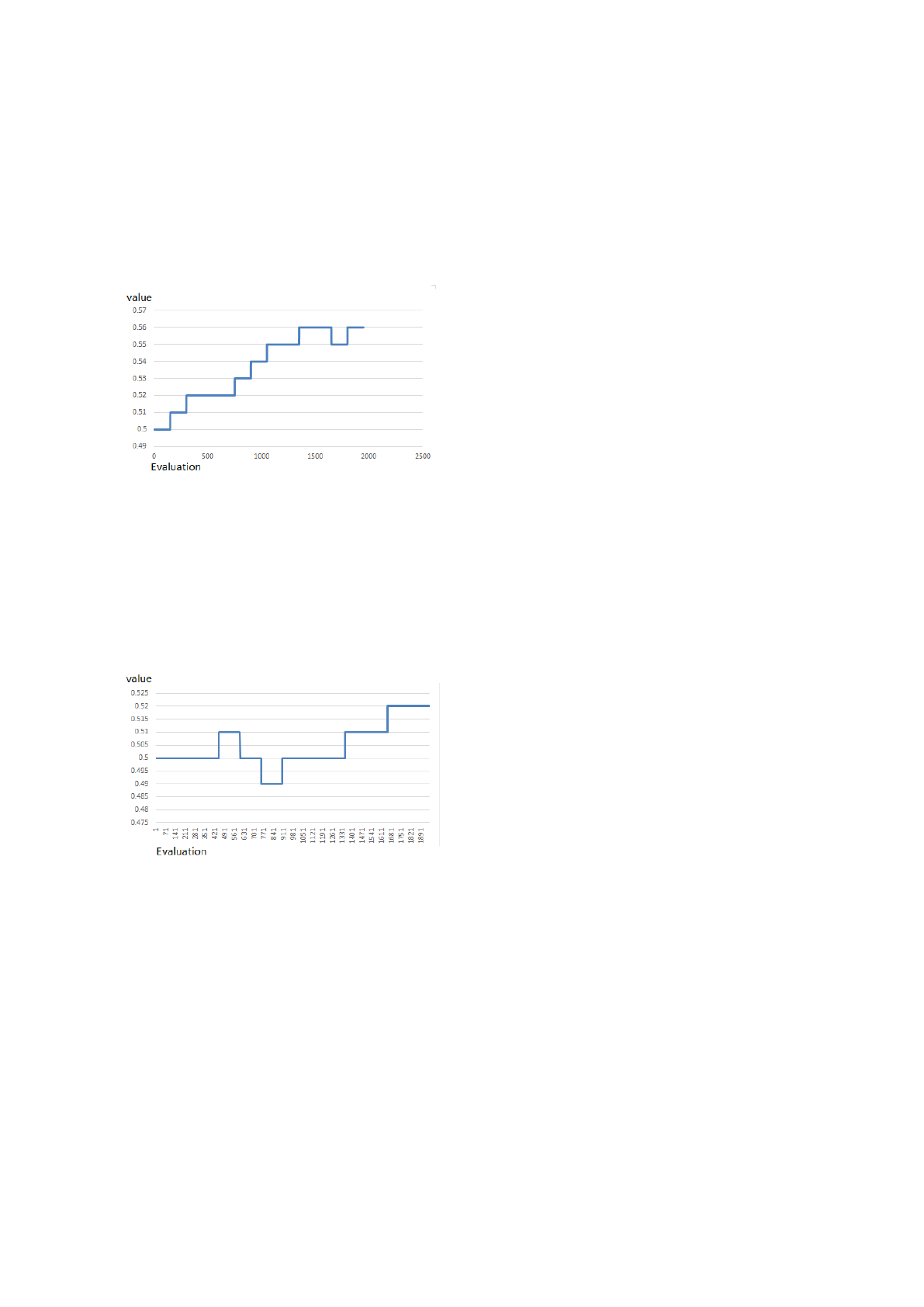
5.3 Evolution of the Parameters

In Fig. 3, we can see the evolution of the scaling fac-

tor (F) during the optimization process. Since the in-

dividuals of the population were similar to each other

at the beginning, the value of F started to increase to

enable big movement in the mutation.

Figure 3: The evolution of the scaling factor F.

In Fig. 4, we can observe the change of the dis-

tribution center (CR

) for the crossover probability

during the process. The value of CR

increased for

the same reason as stated for the scaling factor F, i.e.,

the individuals in the population were similar to each

other. Hence we needed more elements from the mu-

tant vectors to increase the diversity of the population.

Figure 4: The evolution of the distribution center for the

crossover probability.

6 RELATED WORK

DE has been applied successfully in many real ap-

plications such as system design and parameter opti-

mization. In (Sickel et al., 2007) DE and Fast Differ-

ential Evolution (FDE) were employed to solve two

different problems in Power Plant Control. With the

experiments, the authors showed that DE and FDE

outperformed Particle Swarm Optimization (PSO)

and its variants. In (Bakare et al., 2007) comparisons

were made between DE with PSO in the tasks of re-

active control of the power and voltage. The con-

clusion from both (Sickel et al., 2007) and (Bakare

et al., 2007) was that DE outperformed PSO, yet with-

out signiﬁcant superiority. In (Mohanty et al., 2014)

the authors employed DE in the applications of load

frequency control of a multi-source power system.

They proposed the application of DE to optimize P, PI

and PID controllers. However, the running parame-

ters of DE were tuned manually with a trial-and-error

method to achieve good optimization performance.

The main problem with applying DE to solve

practical problems lies in the parameter setting. Very

often domain engineers do not have that knowledge to

decide which parameters to choose for DE. Therefore

it is an appealing idea to enhance DE with some abil-

ity of self-adapting its parameters. The direction of

research has received some efforts recently. In (Gong

and Cai, 2014) multi-strategy adaptive differential

evolution was proposed to locate the best parame-

ters for the model of the proton exchange membrane

fuel cell. Zou et al. (Zou et al., 2011) proposed an

improved Differential Evolution (IDE) with an adap-

tive mutation factor and a dynamical crossover rate

to solve the task assignment problem. In (Mulumba

and Folly, 2012) Self-Adaptive Differential Evolution

(SADE) was used to tune the parameters of a power

system stabilizer (PSS).

7 CONCLUSION

This paper shows that Differential Evolution (DE)

algorithms can be applied successfully to solve the

problem of parameter identiﬁcation in process model-

ing. This is implemented by utilizing DE as a power-

ful global search mechanism to discover best parame-

ters of the model to minimize the difference between

model outputs and true measurement values. Further,

we present a new adaptive DE algorithm that exhibits

two attractive properties for real applications. First,

it does not require prior knowledge about the good

values of the scaling factor and crossover rate for DE.

Second, it enables self-adaptation of these two param-

eters during the running of DE. Case study has been

done of applying this algorithm within the context of

the Furnace Optimized Control System. The results

of the experiments indicate that our new adaptive DE

algorithm outperformed the original DE by yielding

higher accuracy of the models produced.

For future work, we plan to enhance our adaptive

DE algorithm with a more advanced mutation strat-

egy. We also intend to incorporate local search such

as Simplex, Quasi Newton method or some Random

Application of Adaptive Differential Evolution for Model Identiﬁcation in Furnace Optimized Control System

local search methods (Leon and Xiong, 2014b) (Leon

and Xiong, 2015) into the current adaptive DE algo-

rithm. At last, more case studies will be made to ex-

amine our work in more industrial scenarios.

ACKNOWLEDGEMENTS

The work is supported by the Swedish Knowledge

Foundation (KKS) grant (project no 16317).

REFERENCES

Bakare, G., Krost, G., Venayagamoorthy, G., and Aliyu,

U. (2007). Comparative application of differential

evolution and particle swarm techniques to reactive

power and voltage control. In International Confer-

ence on Intelligent Systems Applications to Power Sys-

tems, 2007. ISAP 2007. Toki Messe, Niigata, pages 1–

Gong, W. and Cai, Z. (2014). Parameter optimization of

pemfc model with improved multi-strategy adaptive

differential evolution. Engineering Applications of Ar-

tiﬁcial Intelligence, 27:28–40.

Leon, M. and Xiong, N. (2014a). Investigation of mutation

strategies in differential evolution for solving global

optimization problems. In Artiﬁcial Intelligence and

Soft Computing, pages 372–383. springer.

Leon, M. and Xiong, N. (2014b). Using random local

search helps in avoiding local optimum in diefferential

evolution. In Proc. Artiﬁcial Intelligence and Applica-

tions, AIA2014, Innsbruck, Austria, pages 413–420.

Leon, M. and Xiong, N. (2015). Eager random search for

differential evolution in continuous optimization. In

Progress in Artiﬁcial Intelligence, pages 286–291.

Mohanty, B., Panda, S., and PK, H. (2014). Controller

parameters tuning of differential evolution algorithm

and its application to load frequency control of multi-

source power system. International journal of electri-

cal power & energy systems, 54:77–85.

Mulumba, T. and Folly, K. (2012). Application of self-

adaptive differential evolution to tuning pss parame-

ters. In Power Engineering Society Conference and

Exposition in Africa (PowerAfrica), 2012 IEEE, Jo-

hannesburg, pages 1–5.

Norberg, P. and Leden, B. (1988). New developments of

the computer control system focs-rf - application to

the hot strip mill at ssab, domnarvet. SCANHEATING

II, pages 31–60.

Sickel, J. V., Lee, K., and Heo, J. (2007). Differential evo-

lution and its applications to power plant control. In

International Conference on Intelligent Systems Ap-

plications to Power Systems, 2007. ISAP 2007., Toki

MEsse, Niigata, pages 1–6. IEEE.

Storn, R. and Price, K. (1997). Differential evolution - a

simple and efﬁcient heuristic for global optimization

over continuous spaces. Journal of Global Optimiza-

tion, 11(4):341 – 359.

Xiong, N., Molina, D., Leon, M., and Herrera, F. (2015).

A walk into metaheuristics for engineering optimiza-

tion: Principles, methods, and recent trends. Interna-

tional Journal of Computational Intelligence Systems,

8(4):606–636.

Zou, D., Liu, H., Gao, L., and S.Li (2011). An improved dif-

ferential evolution algorithm for the task assignment

problem. Engineering Applications of Artiﬁcial Intel-

ligence, 24:616–624.

ECTA 2015 - 7th International Conference on Evolutionary Computation Theory and Applications