
Dynamic Obstacle Avoidance using Online Trajectory Time-scaling and
Local Replanning
Ran Zhao
1,2
and Daniel Sidobre
2,3
1
CNRS, LAAS, 7 Avenue du Colonel Roche, F-31400 Toulouse, France
2
Univ. de Toulouse, LAAS, F-31400 Toulouse, France
3
Univ. de Toulouse, UPS, LAAS, F-31400 Toulouse, France
Keywords:
Obstacle Avoidance, Velocity Obstacles, Trajectory Time-scaling, Local Replanning.
Abstract:
In various circumstances, planning at trajectory level is very useful to generate flexible collision-free motions
for autonomous robots, especially when the system interacts with humans or human environment. This paper
presents a simple and fast obstacle avoidance algorithm that operates at the trajectory level in real-time. The
algorithm uses the Velocity Obstacle to obtain the boundary conditions required to avoid a dynamic obstacle,
and then adjust the time evolution using the non-linear trajectory time-scaling scheme. A trajectory local
replanning method is applied to make a detour when the static obstacles block the advance path of the robot,
which leads to failure of implementing time-scaling approach. Cubic polynomial functions are used to describe
trajectories, which brings sufficient flexibility in terms of providing higher order smoothness. We applied this
algorithm on reaching tasks for a mobile robot. Simulation results demonstrate that the technique can generate
collision-free motion in real time.
1 INTRODUCTION
To achieve a large variety of tasks in interaction with
human or human environments, autonomous robots
must have the capability to quickly generate collision-
free motions. Significant research has been per-
formed in the modeling of the path planning problem.
Sample-based planners such as rapidly-exploring ran-
dom trees (RRTs)(LaValle and Kuffner, 2001), or
probabilistic roadmaps (PRMs)(Kavraki et al., 1996)
generate the motion as collision-free paths, which the
robot is expected to follow. They are often fast, but
they generate a global path using an environmental
model and update the planned path when the planned
path is blocked by unmapped obstacles. As a result,
they can not deal with unknown environments with a
large number of dynamic obstacles.
To make the robot more reactive, it is reasonable
to replace paths by trajectories as the interface be-
tween planners and controllers, and to add a trajectory
planner as an intermediate level in the software archi-
tecture. To react to environment changes, the trajec-
tory planning must be done in real time. Meanwhile,
the robot needs to guarantee the human safety and the
absence of collision. So the model for trajectory must
allow fast computation and easy communication be-
tween the different components, including path plan-
ner, trajectory generator, collision checker and con-
troller. To avoid the replan of an entire trajectory, the
model must allow slowing down or deforming locally
a trajectory.
To assure the collision safety of an autonomous
robot in dynamic environment, the velocity of obsta-
cles should be considered when planning the robots
trajectory. The concept of Velocity Obstacle for ob-
stacle avoidance was proposed in (Fiorini and Shillert,
1998) and was later extended to the case of reactive
collision avoidance among multiple robots in (van den
Berg et al., 2011a),(van den Berg et al., 2011b). Ve-
locity obstacles (VOs) represent a subset of the veloc-
ity space where a mobile robot and a dynamic obsta-
cle collide in the future when the mobile robot moves
at a velocity of the VO.
Trajectory time-scaling methods are generally
used to adjust the speed or torque while maintain-
ing the tracking path. The trajectory time-scaling
schemes proposed in (Dahl and Nielsen, 1989) and
(Morenon-Valenzuela, 2006) are used in execution of
fast trajectories along a geometric path, where the
motion is limited by torque constraints. (Szadeczky-
Kardoss and Kiss, 2006) gives an on-line time-scaling
methods based on the tracking error. In this study, we
414
Zhao R. and Sidobre D..
Dynamic Obstacle Avoidance using Online Trajectory Time-scaling and Local Replanning.
DOI: 10.5220/0005570204140421
In Proceedings of the 12th International Conference on Informatics in Control, Automation and Robotics (ICINCO-2015), pages 414-421
ISBN: 978-989-758-123-6
Copyright
c
2015 SCITEPRESS (Science and Technology Publications, Lda.)
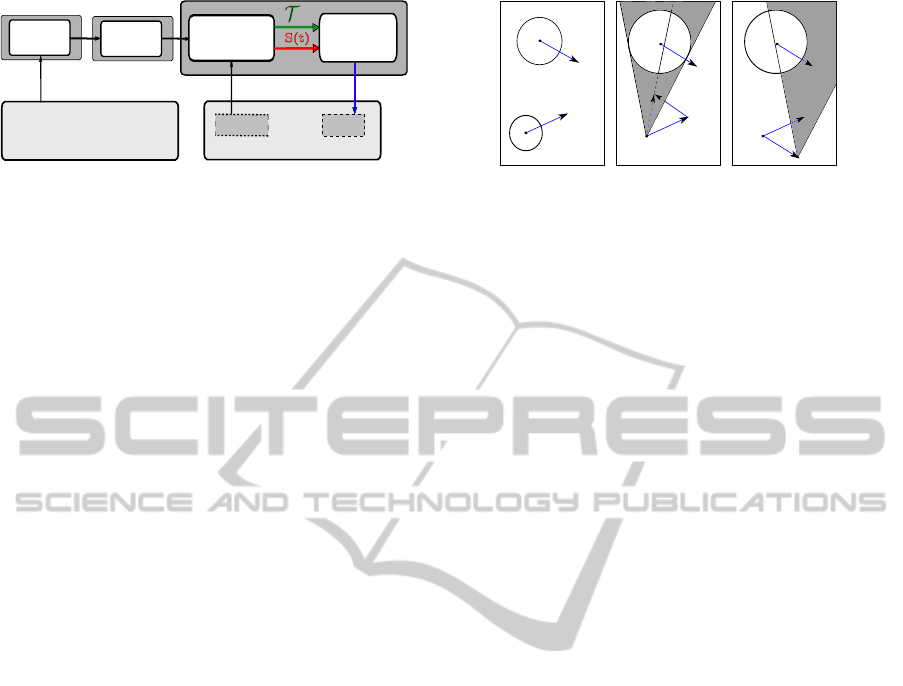
Trajectory
Sensor data
Actuators
ROBOT
Trajectory
planner
Vobs
n
Controller
Path
Planner
Task
Planner
S(t)
Environment
Model
Figure 1: Trajectory planner serves as an intermediate level
between the path planner and the low level controller. The
planner can generate both new trajectories T
n
and time-
scaling functions s(t).
use the trajectory time-scaling schemes to avoid dy-
namic obstacles, which will not result in a change of
path of the robot. Moreover, we apply a non-linear
time-scaling to satisfy the kinematic constraints dur-
ing the collision avoidance.
In this paper, we use a sequence of cubic polyno-
mial functions to describe trajectories and we propose
an efficient obstacle avoidance method in the trajec-
tory level. We build an intermediate level between
the path planner and the low level controller, which
can read sensor information to generate non-linear
time-scaling functions or to replan new trajectories
for avoiding dynamic obstacles, as shown in Fig. 1.
The advantage of our algorithm is more reactive to
dynamically changing environments and temporally
distributes the computations, making it feasible to im-
plement in real-time.
The rest of the paper is organized as follow: We
present the trajectory representations and introduce
notations in Section 2. We describe the obstacle
avoidance algorithms in Section 3 and Section 4. Sim-
ulation results are highlighted in Section 5.
2 NOTATIONS AND
REPRESENTATIONS
2.1 Trajectory Representations
Let C = R
n
denote the n-dimensional configuration
space. A trajectory T can be a direct function of time
or the composition P (u(t)) of a path P (u) and a func-
tion u(t) describing the time evolution along this path.
The background trajectory materials are summarized
in the books from Biagiotti (Biagiotti and Melchiorri,
2008) and Kroger (Kr
¨
oger, 2010). A trajectory T is
then defined as:
T : [t
I
,t
F
] −→ R
n
(1)
t 7−→ T (t)
where T (t) = X(t) = (
1
X(t),
2
X(t),··· ,
n
X(t))
T
in
Cartesian space from the time interval [t
I
,t
F
] to R
n
.
V
a
V
b
A
B
(a)
V
a
V
b
A
B
^
^
V
a
,
b
-V
b
λ
a
,
b
CC
ab
(b)
V
a
A
B
^
^
V
b
VO
b
V
b
(c)
Figure 2: (a) Two circular object with constant velocity. (b)
The collision cone of object A and B, any relative veloc-
ity lies in this cone will cause a collision. (c) The velocity
obstacle V O
b
on the absolute velocity of A.
We choose a particular series of 3
rd
degree poly-
nomial trajectories and name them as Soft Motion tra-
jectories. A Soft Motion trajectory is a type V trajec-
tory defined by Kr
¨
oger(Kr
¨
oger, 2010), which satis-
fies:
V (t) ∈ R
n
|V (t)| ≤ V
max
A(t) ∈ R
n
|A(t)| ≤ A
max
J(t) ∈ R
n
|J(t)| ≤ J
max
(2)
where V , A and J represent the position, velocity, ac-
celeration and jerk, respectively. J
max
,A
max
,V
max
are
the kinematic constraints. Therefore, at a discrete
instant, the trajectory can transfer the motion states
while not exceeding the given motion bounds. The
continuity class of the trajectory is C
2
. For the dis-
cussion of the next sections, a state of motion at an
instant t
i
is denoted as M
i
= (X
i
,V
i
,A
i
).
2.2 Velocity Obstacle (VO)
A VO (Fiorini and Shillert, 1998) represents a set of
velocities that create an obstacle collision. Consider
two circular objects A and B, shown in Fig. 2(a) at
time t
0
, with constant velocity v
a
and v
b
. Let circle
A represent the robot, and B represent the obstacle.
The point
b
A is center of circle A,
b
B is mapped by
enlarging B by the radius of A, shown in Fig. 2(b).
The Collision Cone CC
a,b
is then defined as the set of
colliding relative velocities between
b
A and
b
B:
CC
a,b
=
n
v
a,b
|λ
a,b
\
b
B =
/
0
o
(3)
where v
a,b
is the relative velocity of
b
A with respect to
b
B, v
a,b
= v
a
− v
b
, and λ
a,b
is the line of v
a,b
.
The shape of CC
a,b
is the planar sector with apex
in
b
A, bounded by the two tangent from
b
A to
b
B. Any
relative velocity lies in this cone will cause a colli-
sion. To deal with multiple obstacles, it is interesting
to consider the VO of the absolute veloctiy of A, This
DynamicObstacleAvoidanceusingOnlineTrajectoryTime-scalingandLocalReplanning
415

can be done simply by adding the velocity of B:
VO
b
= CC
a,b
⊕ v
b
(4)
where ⊕ is the Minkowski sum. When the velocity of
robot A is included in the VO
b
, the robot will collide
with obstacle B in the future. In the case of multiple
obstacles, the collision-free velocity can be obtained
by selecting a velocity that is not contained in any VO.
Fig. 2(c) shows an illustration of an VO.
3 COLLISION AVOIDANCE BY
TRAJECTORY TIME-SCALING
3.1 Time-scaling Function
A time-scaling function s = s(t) is an increasing func-
tion of time. Using the time-scaling function a new
trajectory
e
T (t) can be defined such that
e
T (t) = T (s).
Applying the time scaling function does not change
the path taken by the robot, but brings the following
changes in the velocity and acceleration profile of the
trajectory.
e
V (t) = V (s) ˙s (5)
e
A(t) = A(s) ˙s
2
+V (s)¨s (6)
e
J(t) = J(s) ˙s
3
+ 3A(s) ˙s ¨s +V (s)
...
s
(7)
where s(t) scales up the velocity and acceleration for
s(t) > 1 and scales it down for s(t) < 1.
In this current work, we use the concept of the Op-
timal Motion to describe the time variation. The Opti-
mal Motion is a motion with jerk, acceleration and ve-
locity constraints successively saturated (Herrera and
Sidobre, 2005). We use the velocity of an Optimal
Motion to represent the time variaiton. In this case,
we are able to control the time change by defining the
maximum jerk J
max
, acceleration A
max
and velocity
V
max
, thus the motion of the robot can be bounded,
e.g. the kinematic constraints (J
max
, A
max
, V
max
) of
the robot motion are linked to the Coefficient of the
time-scaling function (J
max
, A
max
, V
max
). So we use a
non-linear time-scaling function as follow:
s(t) =
s(t)
i
+ At + J
t
2
2
, J = −J
max
s(t)
i
+ At, J = 0,A = A
max
s(t)
i
+ At + J
t
2
2
, J = J
max
(8)
In this study, we assumed that a mobile service robot
should not increase its speed to avoid moving ob-
stacles, because it could cause some people anxiety.
Thus V
max
= 1. It also should be noted that the
acceleration/de-acceleration produced by the scaling
transformation must respect the acceleration and jerk
bounds and hence the following inequalities are ob-
tained: |
e
V (t)| ≤ V
max
, |
e
A(t)| ≤ A
max
, |
e
J(t)| ≤ J
max
.
With the framework for constructing scaling function
in place, the collision avoidance problem becomes of
choosing what scaling function to use for the robot at
any given instant.
3.2 Single Obstacle Case
The case of a robot avoiding a moving obstacle is
first considered. This is illustrated in Fig. 2(c) which
shows robot A in collision course with passively mov-
ing obstacle B. Collision is avoided if the veloc-
ity of A is out of VO
b
: v
a
≤ v
max
, where v
max
is
the maximum velocity of A on the VO
b
boundary.
With the trajectory of robot, we could get the final
value of the time-scaling function s(t)
f
which satisfy
that: v
a
(s) ≤ v
max
. Then we could define a Opti-
mal Motion for the time-scaling function. The ini-
tial condition and final condition of the motion are
(0,0, s(t)
c
) and (1,0,s(t)
f
), respectively. s(t)
c
is the
current time-scaling factor when the robot start to ac-
celerate/decelerate. [0, T
op
] is the time interval of the
time-scaling function, where T
op
is the execution time
of the Optimal Motion . So J, A and s(t) are piecewise
functions:
J(t) =
−J
max
0
J
max
A(t) =
−J
max
t
−A
max
−A
max
+ J
max
t
2
2
(9)
s(t) =
s(t)
c
+ A(t)t −J
max
t
2
2
t ∈ [0,
A
max
J
max
]
s(t)
c
+ A
max
t t ∈ [
A
max
J
max
,T
op
−
A
max
J
max
]
s(t)
c
+ A(t)t +J
max
t
2
2
t ∈ [T
op
−
A
max
J
max
,T
op
]
(10)
Then from the Eqs 5-10, we can caculate the maximum
coefficients, J
max
and A
max
, of the time-scaling func-
tion.
3.3 Multiple Obstacles Case
In the case of many obstacles, it may be useful to pri-
oritize the obstacles so that those with imminent col-
lision will take precedence over those with long time
to collision. We use the concept of imminent (Fiorini
and Shillert, 1998) which is a collision between the
robot and an obstacle if it occurs at some time t < T
h
,
where T
h
is a suitable time horizon, selected based on
system dynamics, obstacle trajectories, and the com-
putation rate of the avoidance maneuvers. To account
for imminent collisions, we compute the distance d
ICINCO2015-12thInternationalConferenceonInformaticsinControl,AutomationandRobotics
416

between the robot A and an obstacle B at time instant
t. If the d < v
a,b
∗ T
h
, we treat B as a imminent col-
lision and the avoidance procedure will be first con-
sidered. If not, even v
a
lies inside the VO region, the
old time evolution will be maintained. If there ex-
ist many imminents, the minimal time-scaling factor
s(t)
f
will be applied to the original trajectory. Al-
gorithm 1 shows the overall pseudocode of collision
avoidance for multiple obstacles.
Algorithm 1: Trajectory time-scaling Based Collision
Avoidance.
Input: a trajectory T of robot A, number of obsta-
cles M, T
h
1: for i = 0 to M do
2: Obtain the VO
i
, v
a
on T at time t
3: if v
a
T
VO
i
6=
/
0 then
4: Compute the relative velocity v
i
between the
robot and the obstacle i
5: Compute the distance d
i
between the robot
and the obstacle i
6: if d
i
< v
i
∗ T
h
then
7: Calculate the time-scaling factor s(t)
f i
for
the single obstacle
8: else
9: s(t)
f
= s(t)
c
10: end if
11: end if
12: end for
13: return the minimal factor s(t)
f min
, then compute
the coefficients J
max
and A
max
4 COLLISION AVOIDANCE BY
TRAJECTORY LOCAL
REPLANNING
The global path planning method considers the sur-
rounding environment knowledge, and then attempts
to optimize the path. However, some problems are
existing in this method such as data are incomplete,
the real environment situations are unexpected and the
real-time operation of the robot.
Autonomous robots often operate in human envi-
ronment where the obstacles may block the robot’s
path. For example, an obstacle may have the same
path with the robot but with a very low velocity, or
an obstacle moves on the robot’s path and then halts
there. In the first case, the time-scaling function will
return a extreme small value, which leads to a quite
slow robot motion. In the second case, the time-
scaling function will stop the robot and goal position
cannot be reached. Thus, the robot needs to be able to
V
a
Goal
P
m
P
r
B
V
b
VO
A
^
r
a
Figure 3: Choice of the middle and return waypoints for
trajectory replanning.
replan quickly as the knowledge of the environment
changes. This can be done simply by adding a middle
waypoint where the robot can pass through to avoid
the obstacle. Fig. 3 illustrates a situation of the first
case. Robot A and the obstacle B have the same path
P (u) while V
b
is small. To replan a new trajectory, we
need to find a middle waypoint P
m
to make a detour,
and a return point P
r
to go back the original path.
To avoid the obstacle, the middle waypoint must
be out of VO. Waypoint on the boundaries of VO
would result in A grazing B. For sake of simplicity,
we can enlarge the VO region slightly by increase the
radius of
b
B by a constant r (the black dashed circle in
Fig. 3). In this study, we choose P
r
as:
P
r
=
b
B
\
P (u)
B
⊕ r
a
v
a,b
|v
a,b
|
(11)
where P(u)
B
is part of the path P (u) that is behind
the obstacle B. Then the middle waypoint P
m
is the
point of intersection between the two tangents λ
b
A,
b
B
and λ
P
r
,
b
B
.
4.1 Trajectory Generation Through
Waypoints
Now the problem becomes to generate a trajectory
that traverse these waypoints. We consider a solu-
tion to plan point-to-point (straight-line) trajectories
that halt at each via-point where the direction of the
path changes. Then we smooth the edges of the tra-
jectory to produce smoother motion defined by kine-
matics conditions.
The first step is to convert a piecewise linear
path to a time-optimal trajectory that stops at each
waypoint. The trajectory along a straight-line path
should be a phase-synchronized motion(Broquere
et al., 2008). To achieve that, we compute the final
time for each dimension. Considering the largest mo-
tion time, we readjust the other dimension motions
to this time. Time adjusting is done by decreasing
linearly J
max
,A
max
,V
max
. In other words, the motion
consumes minimum time for one direction. At other
directions, the motions are conditioned by the mini-
mum one.
The point-to-point (straight-line) trajectory T
pt p
obtained in the first step is feasible, but is not sat-
DynamicObstacleAvoidanceusingOnlineTrajectoryTime-scalingandLocalReplanning
417

P
r
P
m
A
B
P
start
P
end
ε
ε
v
l
start
l
end
n
i
n
i+1
P
(t
I
+t
F
)/2
P
s
Figure 4: Error between the smoothed trajectory and pre-
planed path.
isfactory because the velocity varies greatly at each
waypoint, which stops the motion. These stops can
be avoided by drawing shortcuts between random
points on the trajectory. Without loss of generality
we consider three adjacent points (P
s
,P
m
,P
r
) and the
smoothing at the intermediate via-point P
m
. Firstly,
the two straight-line trajectories T
P
s
P
m
and T
P
m
P
r
are
computed respectively. Then we choose two points
(P
start
,P
end
) based on the parameter l, which is the
distance from the point P
m
on the trajectory. Then
we compute a trajectory to connect P
start
and P
end
.
(l
start
,l
end
) are used to denote the two distances and
they defines the limits of the smoothed area. The pos-
sible choices of these two points are infinite, and the
resulting trajectories can vary greatly due to the differ-
ent choices. In this study, we choose the two points
considering the distance between the trajectory and
the obstacle. We discuss how to choose the points in
this paragraph and then detail the smooth trajectory
generation in the next part.
Considering the case of three adjacent points
P
s
,P
m
,P
r
, see Fig.4,
−→
n
i
being the normal unit vectors
to the straight line P
s
P
m
, and T
s
(t) the smoothed tra-
jectory. Then the error ε can be defined as:
ε(t) = min
t∈[t
I
,t
F
]
([T
s
(t) − P
m
] ·
−→
n
i
,[T
s
(t) − P
m
] ·
−−→
n
i+1
)
ε = max(ε(t)) (12)
To compute this error, we introduce another parame-
ter ε
v
, which is represented by the minimum distance
between the vertex P
i
and the trajectory T
s
(t):
ε
v
= min
t∈[t
I
,t
F
]
d(P
i
,T
s
(t)) (13)
As the start and end points of the blend we choose
locate at the symmetric segments on each straight-line
trajectory, the error E
v
happens at the bisector of the
angle α formed by the 3 adjacent points, Therefore,
ε
v
= d(P
m
,T
t
I
+t
F
2
) (14)
ε = ε
v
∗ sin
α
2
(15)
To avoid the collision, a simple possibility is to
change the distance l to make the error satisfy that:
ε < d
(p
m
,B)
− r
A
(16)
where d
(p
m
,B)
is the distance between the point P
m
and
the obstacle B. To achieve Eq. 16 we introduce a
parameter δ, for a general case, it is defined as:
δ =
l
start
|P
s
P
m
|
=
l
end
|P
m
P
r
|
(17)
Thus δ ∈ [0,1]. Then we can compute in a loop and
get the δ
max
.
4.2 Smooth Trajectory Generation
In this part, we describe how to generate a smooth
motion to connect P
start
and P
end
. The motion state
of these two points are M
s
and M
e
respectively. Since
each aixs variable is assumed to be independent, the
minimum execution time between M
s
and M
e
is de-
termined by the slowest single-aixs trajectory. Then
the motion on the rest of the axis must be interpo-
lated to this imposed time which is called T
imp
. More
precisely, f (M
s
,M
e
,J
max
,A
max
,V
max
) is used to com-
pute the time of the time-optimal interpolant between
motion states M
s
and M
e
under the kinematic bounds
J
max
, A
max
and V
max
. Thus,
T
imp
= max( f (M
j
s
,M
j
e
,J
j
max
,A
j
max
,V
j
max
)) j ∈ [1,n]
The interpolation problem becomes one of building a
motion with predefined time. We propose three meth-
ods by computing different parameters of the trajec-
tory.
Three-segment Interpolants. If we consider states
M
s
and M
e
defined by a starting instant t
s
and an end-
ing instant t
e
, the starting and ending situations to be
connected are: (X
s
,V
s
,A
s
) and (X
e
,V
e
,A
e
). An inter-
esting solution to connect this portion of trajectories is
to define a sequence of three trajectory segments with
constant jerk that bring the motion from the initial sit-
uation to the final one within time T
imp
. We choose
three segments because we need a small number of
segments and there is not always a solution with one
or two segments.
The system to be solved is then defined by 13 con-
straints: the initial and final situations (6 constraints),
the continuity in position velocity and acceleration for
the two switching situations and time. Each segment
of a trajectory is defined by four parameters and time.
If we fix the three durations T
1
= T
2
= T
3
=
T
imp
3
,
we obtain a system with 13 parameters where only
the three jerks are unknown(Broqu
`
ere and Sidobre,
2010). As the final control system is periodic with
period T , the time T
imp
/3 must be a multiple of the
period T , and in this study, T
imp
is chosen to be a mul-
tiple of 3T .
ICINCO2015-12thInternationalConferenceonInformaticsinControl,AutomationandRobotics
418
Three-segment Interpolants with Bounded Jerk.
The three-segment interpolants solves the problem of
trajectory generation with fixed duration for each seg-
ment. However, it cannot be guaranteed that the com-
puted jerk is always bounded. Here, we introduce a
variant three-segment method with defined jerk.
Same as the three-segment method, the system
is also defined by 13 constraints. With the variant
method, however, we fix the jerks on the first and third
segments as
|
J
1
|
=
|
J
3
|
, which have the value bounded
within the kinematic constraints. Then, the unknown
parameters in the system are J
2
and the three time du-
rations. Thus we obtain a system of four equations
with four parameters (J
2
, T
1
, T
2
and T
3
):
A
e
= J
3
T
3
+ A
2
(18)
V
e
= J
3
T
2
3
2
+ A
2
T
3
+V
2
(19)
X
e
= J
3
T
3
3
6
+ A
2
T
2
3
2
+V
2
T
3
+ X
2
(20)
T
imp
= T
1
+ T
2
+ T
3
(21)
where
A
2
=J
2
T
2
+ J
1
T
1
+ A
s
V
2
=J
2
T
2
2
2
+ (J
1
T
1
+ A
s
)T
2
+ J
1
T
2
1
2
+ A
s
T
1
+V
s
X
2
=J
2
T
3
2
6
+ (J
1
T
1
+ A
s
)
T
2
2
2
+ (J
1
T
2
1
2
+ A
s
T
1
+V
s
)T
2
+ J
1
T
3
1
6
+ A
s
T
2
1
2
+V
s
T
1
+ X
s
To choose the values of jerks on each dimension, we
resort to the velocities V
s
and V
e
. The jerks are fixed
by J
1
= −J
3
= J
max
when V
s
−V
e
> 0, and by J
1
=
−J
3
= −J
max
when V
s
−V
e
< 0. If V
s
−V
e
= 0, we
compare the values of A
s
and A
e
instead.
Jerk-bounded, Acceleration-bounded, Velocity-
bounded Interpolants. Now we derive the all-
bounded trajectory given a fixed duration T
imp
. The
method in the previous paragraph can directly bound
the jerk, but have to readjust the jerk values by a pre-
defined resolution to bound the velocity and accelera-
tion. As we detect the longest execution time T
imp
by
computing the time-optimal trajectory on each aixs,
the jerk is saturated and the acceleration and velocity
may be saturated, depending on different cases. Thus,
we can extend the duration of all axis (except the one
with the longest duration) to T
imp
by unsaturated in-
terpolants while maintaining the number of segments
N
j
on each aixs. We name it a Slowing Down Motion.
Algorithm 2 shows the generation of all-bounded in-
terpolants.
Algorithm 2: All-Bounded Interpolants Generation.
Input: Motion states: M
s
, M
e
; number of DOFs: n;
T
imp
Output: Jerk-Bounded, Acceleration-Bounded,
Velocity-Bounded Interpolants
1: for j = 1 to n do
2: Compute the time-optimal interpolants between
M
s
and M
e
, then get the execution time T
j
3: Get N
j
and the execution time on each segment
T
N
j
4: if N
j
= 0 then
5: No motion on this axis, maintain the time-
optimal interpolants
6: else
7: Enlarge T
N
j
by T
N
j
= T
N
j
+
T
imp
−T
j
N
j
8: Compute the new Jerk on each segment J
N
j
9: end if
10: Generate the interpolants with J
N
j
and T
N
j
11: end for
0 1 2 3 4 5 6 7 8 9 10 11
−1
−0.5
0
0.5
1
X (m)
Y (m)
Robot
O
1
(a) t = 0 s
0 1 2 3 4 5 6 7 8 9 10 11
−1
−0.5
0
0.5
1
X (m)
Y (m)
Robot
O
1
(b) t = 3 s
0 1 2 3 4 5 6 7 8 9 10 11
−1
−0.5
0
0.5
1
X (m)
Y (m)
Robot
O
1
(c) t = 6 s
0 1 2 3 4 5 6 7 8 9 10 11
−1
−0.5
0
0.5
1
X (m)
Y (m)
Robot
O
1
(d) t = 7.51 s
0 1 2 3 4 5 6 7 8 9 10 11
−1
−0.5
0
0.5
1
X (m)
Y (m)
Robot
O
1
(e) t = 0 s
0 1 2 3 4 5 6 7 8 9 10 11
−1
−0.5
0
0.5
1
X (m)
Y (m)
Robot
O
1
(f) t = 3 s
0 1 2 3 4 5 6 7 8 9 10 11
−1
−0.5
0
0.5
1
X (m)
Y (m)
Robot
O
1
(g) t = 6 s
0 1 2 3 4 5 6 7 8 9 10111213
−1
−0.5
0
0.5
1
X (m)
Y (m)
Robot
O
1
(h) t = 9.21 s
Figure 5: A robot avoids an obstacle that is moving along
the same trajectory as the robot (a)-(d): The original tra-
jectory collides with the obstacle at 6-7.51 s, (e)-(h): The
scaled collision-free trajectory.
0 1 2 3 4 5 6 7 8 9
0.6
0.7
0.8
0.9
1
Time (s)
S(t) (m)
(a)
0 1 2 3 4 5 6 7 8 9
−9
−6
−3
0
3
6
9
Time (s)
Value
Position (m)
Velocity (m/s)
Acceleration (m/s
2
)
jerk (m/s
3
)
(b)
Figure 6: Time-scaling function and scaled trajectory of
Fig. 5. (a): Time-scaling function, (b): position, velocity,
acceleration and jerk profile of the scaled trajectory along
X axis.
5 SIMULATION RESULTS
The initial trajectories from start (0,0) to the goal
(10,0) for the robots were obtained by modeling the
robots as unicycle. The maximum velocity, accelera-
tion and jerk of the robot was set to 1.5 m/s, 3 m/s
2
and 9 m/s
3
, respectively.
DynamicObstacleAvoidanceusingOnlineTrajectoryTime-scalingandLocalReplanning
419
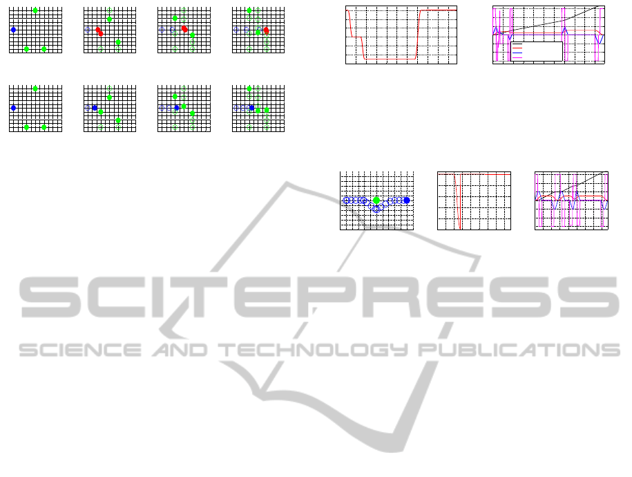
0 1 2 3 4 5 6 7 8 9 10 11
−5
−4
−3
−2
−1
0
1
2
3
4
5
X (m)
Y (m)
Robot
O
1
O
2
O
3
(a) t = 0 s
0 1 2 3 4 5 6 7 8 9 10 11
−5
−4
−3
−2
−1
0
1
2
3
4
5
X (m)
Y (m)
Robot
O
1
O
2
O
3
(b) t = 2 s
0 1 2 3 4 5 6 7 8 9 10 11
−5
−4
−3
−2
−1
0
1
2
3
4
5
X (m)
Y (m)
Robot
O
1
O
2
O
3
(c) t = 4 s
0 1 2 3 4 5 6 7 8 9 10 11
−5
−4
−3
−2
−1
0
1
2
3
4
5
X (m)
Y (m)
Robot
O
1
O
2
O
3
(d) t = 5 s
0 1 2 3 4 5 6 7 8 9 10 11
−5
−4
−3
−2
−1
0
1
2
3
4
5
X (m)
Y (m)
Robot
O
1
O
2
O
3
(e) t = 0 s
0 1 2 3 4 5 6 7 8 9 10 11
−5
−4
−3
−2
−1
0
1
2
3
4
5
X (m)
Y (m)
Robot
O
1
O
2
O
3
(f) t = 2 s
0 1 2 3 4 5 6 7 8 9 10 11
−5
−4
−3
−2
−1
0
1
2
3
4
5
X (m)
Y (m)
Robot
O
1
O
2
O
3
(g) t = 4 s
0 1 2 3 4 5 6 7 8 9 10 11
−5
−4
−3
−2
−1
0
1
2
3
4
5
X (m)
Y (m)
Robot
O
1
O
2
O
3
(h) t = 5 s
Figure 7: A robot avoids multiple obstacle. (a)-(d): The
original trajectory collides with all the obstacles, (e)-(h):
The scaled collision-free trajectory.
5.1 Single Obstacle Avoidance
Fig. 5 shows the simulation results for an obstacle
moving along the path of the robot. The blue and
green circles represent the robot and the obstacle re-
spectively. The situation shown in Fig. 5 takes place
when the robot moves along a corridor. The obstacle
moves at a velocity of vx = 1 m/s from the initial lo-
cation (3,0). As shown in Fig. 5(a)-5(d), the robot
collides with the obstacle at 6-7.51 s. Fig. 5(e)-5(h)
demonstrates the time-scaled results. Obstacle avoid-
ance was achieved by decelerating the robot. The du-
ration of the trajectory was extended to 9.21 s. Fig.
6 illustrates the time-scaling function and scaled tra-
jectory along the X axis. Results show that the robot
decelerated to a safety velocity very fast (in less than
1 s), and all kinematic variables were well bounded
during the construction of the scaled trajectory.
5.2 Multiple Obstacles Avoidance
Fig. 7 depicts a multiple collision situation. The ob-
stacles O
1
, O
2
and O
3
moved at a velocity of vy = 2
m/s, -1.15 m/s and 0.9 m/s, and started at the loca-
tion (3,-5), (5,5), and (7,-5), respectively. The robot
collided with the three obstacles at t = 2 s, t = 4 s
and t = 5 s respectively when it followed the origi-
nal trajectory. The trajectory was scaled at t = 0.3
s to pass obstacle O
1
through the trajectory, and was
scaled at t = 1.5 s to avoid O
2
. After the second time-
scaling function, the VO became an empty set, then
the system switch to the original trajectory by setting
s(t) = 1. Fig. 8 shows the time-scaling function and
the time-scaled trajectory.
5.3 Trajectory Replanning
Fig. 9 describes the obstacle avoidance using trajec-
tory replanning. The time-scaling function returned to
0 because the velocity of the robot always lied in VO.
0 1 2 3 4 5 6 7 8 9 10
0.4
0.5
0.6
0.7
0.8
0.9
1
Time (s)
S(t) (m)
(a)
0 1 2 3 4 5 6 7 8 9 10
−9
−6
−3
0
3
6
9
Time (s)
Value
Position (m)
Velocity (m/s)
Acceleration (m/s
2
)
jerk (m/s
3
)
(b)
Figure 8: Time-scaling function and scaled trajectory of
Fig. 7. (a): Time-scaling function, (b): position, velocity,
acceleration and jerk profile of the scaled trajectory along
X axis.
0 1 2 3 4 5 6 7 8 9 10 11
−5
−4
−3
−2
−1
0
1
2
3
4
5
X (m)
Y (m)
Robot
O
1
(a)
0 1 2 3 4 5 6 7 8
0
0.2
0.4
0.6
0.8
1
Time (s)
S(t) (m)
(b)
0 1 2 3 4 5 6 7 8
−9
−6
−3
0
3
6
9
Time (s)
Value
(c)
Figure 9: Simulation of trajectory local replanning. (a): The
final path of the robot, (b): Time-scaling function, (c): The
kinematic profile of the replanned trajectory along X axis.
The system replanned a new trajectory when s(t) = 0
and s(t) was set to 1 immediately while the new tra-
jectory was executed. Fig. 9(a)-9(c) illustrates the
robot path, time-scaling function and the kinematic
variables, respectively.
6 CONCLUSIONS AND FUTURE
WORKS
This paper presents a simple and fast obstacle avoid-
ance algorithm that operates at the trajectory level in
real-time. It uses the trajectory time-scaling functions
and trajectory replanning scheme to compute C
2
tra-
jectories that are bounded in velocity, acceleration and
jerk. The proposed algorithm is based on the use of
pre-planned trajectories. The Velocity Obstacle con-
cept was used to obtain the boundary conditions re-
quired to avoid a dynamic obstacle. The simulation
results validate the effectiveness of this algorithm to
deal with typical collision states within a short pe-
riod of time. Future work will include extending the
trajectory time-scaling scheme to the robot manipu-
lators. Real-time collision-free trajectory planning is
more complex for many-DOFs manipulators because
time-scaling functions should be considered for each
joint. Velocity Obstacle are not suitable anymore and
new criterions for collision boundary conditions must
be implemented.
ICINCO2015-12thInternationalConferenceonInformaticsinControl,AutomationandRobotics
420

REFERENCES
Biagiotti, L. and Melchiorri, C. (2008). Trajectory Planning
for Automatic Machines and Robots. Springer.
Broqu
`
ere, X. and Sidobre, D. (2010). From motion plan-
ning to trajectory control with bounded jerk for ser-
vice manipulator robots. In IEEE Int. Conf. Robot.
And Autom.
Broquere, X., Sidobre, D., and Herrera-Aguilar, I. (2008).
Soft motion trajectory planner for service manipula-
tor robot. Intelligent Robots and Systems, 2008. IROS
2008. IEEE/RSJ International Conference on, pages
2808–2813.
Dahl, O. and Nielsen, L. (1989). Torque limited path fol-
lowing by on-line trajectory time scaling. In Robotics
and Automation, 1989. Proceedings., 1989 IEEE In-
ternational Conference on, pages 1122–1128 vol.2.
Fiorini, P. and Shillert, Z. (1998). Motion planning in dy-
namic environments using velocity obstacles. Inter-
national Journal of Robotics Research, 17:760–772.
Herrera, I. and Sidobre, D. (2005). On-line trajectory plan-
ning of robot manipulators end effector in cartesian
space using quaternions. In 5th Int. Symposium on
Measurement and Control in Robotics.
Kavraki, L., Svestka, P., Latombe, J.-C., and Overmars, M.
(1996). Probabilistic roadmaps for path planning in
high-dimensional configuration spaces. Robotics and
Automation, IEEE Transactions on, 12(4):566–580.
Kr
¨
oger, T. (2010). On-Line Trajectory Generation in
Robotic Systems, volume 58 of Springer Tracts in Ad-
vanced Robotics. Springer, Berlin, Heidelberg, Ger-
many, first edition.
LaValle, S. M. and Kuffner, J. J. (2001). Randomized
kinodynamic planning. The International Journal of
Robotics Research, 20(5):378–400.
Morenon-Valenzuela, J. (2006). Tracking control of on-line
time-scaled trajectories for robot manipulators under
constrained torques. In Robotics and Automation,
2006. ICRA 2006. Proceedings 2006 IEEE Interna-
tional Conference on, pages 19–24.
Szadeczky-Kardoss, E. and Kiss, B. (2006). Tracking error
based on-line trajectory time scaling. In Intelligent
Engineering Systems, 2006. INES ’06. Proceedings.
International Conference on, pages 80–85.
van den Berg, J., Guy, S., Lin, M., and Manocha, D.
(2011a). Reciprocal n-body collision avoidance. In
Pradalier, C., Siegwart, R., and Hirzinger, G., editors,
Robotics Research, volume 70 of Springer Tracts in
Advanced Robotics, pages 3–19. Springer Berlin Hei-
delberg.
van den Berg, J., Snape, J., Guy, S., and Manocha,
D. (2011b). Reciprocal collision avoidance with
acceleration-velocity obstacles. In Robotics and Au-
tomation (ICRA), 2011 IEEE International Confer-
ence on, pages 3475–3482.
DynamicObstacleAvoidanceusingOnlineTrajectoryTime-scalingandLocalReplanning
421
