Application of Sensory Body Schemas to Path Planning

for Micro Air Vehicles (MAVs)

Eniko T. Enikov

and Juan-Antonio Escareno

Department of Aerospace and Mechanical Engineering, University of Arizona,

1130 N. Mountain Ave, Tucson, AZ 85721, U.S.A.

Directorate for Research and Innovation (DRII), Institut Polytechnique des Sciences Avanc

ees (IPSA),

7-9 Rue Maurice Grandcoing, Ivry-sur-Seine, 94200, France

Keywords:

Micro-Air Vehicles, Artiﬁcial Neural Network, Path Planning, Body Schema, Cognitive Robotics.

Abstract:

To date, most autonomous micro air vehicles (MAV-s) operate in a controlled environment, where the location

of and attitude of the aircraft are measured be dedicated high-power computers with IR tracking capability. If

MAV-s are to ever exit the lab and carry out autonomous missions, their ﬂight control systems needs to utilize

on-board sensors and high-efﬁciency attitude determination algorithms. To address this need, we investigate

the feasibility of using body schemas to carry out path planning in the vision space of the MAV. Body schemas

are a biologically-inspired approach, emulating the plasticity of the animal brains, allowing efﬁcient represen-

tation of non-linear mapping between the body conﬁguration space, i.e. its generalized coordinates and the

resulting sensory outputs. This paper presents a numerical experiment of generating landing trajectories of

a miniature rotor-craft using the notion of body and image schemas. More speciﬁcally, we demonstrate how

a trajectory planning can be executed in the image space using a pseudo-potential functions and a gradient-

based maximum seeking algorithm. It is demonstrated that a neural-gas type neural network, trained through

Hebbian-type learning algorithm can learn a mapping between the rotor-craft position/attitude and the output

of its vision sensors. Numerical simulations of the landing performance of a physical model is also presented,

The resulting trajectory tracking errors are less than 8 %.

1 INTRODUCTION

The applications of Miniature Air Vehicles (MAVs)

have widely diversiﬁed during the last ﬁve years.

They comprise both military and civilian, though the

latter has had a lower development rate. The main

goal of unmanned air vehicles (UAVs) is to provide a

remote and mobile extension of human perceptions,

allowing not only the security of the user (soldier,

policeman, cameraman, volcanologist), but also the

collection of valuable information of zones/targets of

interest used for on-line or off-line analysis. Ro-

torcraft MAVs represent an excellent alternative due

to their versatile ﬂight proﬁle as hovering, vertical

take-off/landing (VTOL) and maneuverability, allow-

ing the access to small enclosures and navigation

within unstructured environments. The enhanced pro-

ﬁciency of recently developed navigation and control

algorithms has brought about the possibility of using

VTOL MAVs in other civilian applications such as

wildlife studies, urban surveillance (car and pedes-

trian trafﬁc), and pollution monitoring, to mention

just a few.

Despite the great number of potential MAV-based

applications, the operational role of these air robots

remains limited to being passive agents during their

missions such as in surveillance tasks. Enhancing the

current proﬁle of MAVs implies endowing them with

the ability to perform autonomous decision making,

for example, an ability to establish a landing site, nav-

igate to it, and land/perch. To date, almost all MAV

research is carried out in a controlled laboratory en-

vironment where both the target landing location, as

well as the MAV position are measured in real-time

using a complex IR vision tracking system. If MAVs

are ever to exit the lab, their ﬂight control needs to

be autonomous and based on on-board image and al-

titude sensors. To address this need, we proposed to

utilize a biologically inspired approach emulating the

plasticity of avian and human brain.

Traditionally, MAV controllers are derived from

linearized models of the vehicle. The stability of these

Enikov E. and Escareno J..

Application of Sensory Body Schemas to Path Planning for Micro Air Vehicles (MAVs).

DOI: 10.5220/0005547000250031

In Proceedings of the 12th International Conference on Informatics in Control, Automation and Robotics (ICINCO-2015), pages 25-31

ISBN: 978-989-758-122-9

 2015 SCITEPRESS (Science and Technology Publications, Lda.)

controllers is therefore limited to relatively small roll

and pitch angles, while in the case of fast maneuvers,

it is not guaranteed. Machine learning techniques

have been successful in learning models based on data

from human pilots (Abbeel et al., 2007), in improving

performance of control using reinforcement learning

(Lupashin et al., 2010), and exploring aggressive ma-

neuvers such as fast translation and back ﬂip (Purwin

and D’Andrea, 2009; Gillula et al., 2011). In con-

trast to these prior efforts, the approach proposed here

does not simply replicate the control of human oper-

ators, rather, it is based on the premise that through

self-learning, the robot can create its own representa-

tion of its body and vision system and, upon a period

of training, can learn to perform such maneuvers on

its own. More speciﬁcally, we demonstrate the ap-

plication of an artiﬁcial neural network representa-

tion of the robot’s vision and attitude systems capa-

ble of controlling the robot to a target landing site.

The property of ANN to provide control laws through

implicit inversion of the robot’s kinematic chain or in

our case the non-linear transformation between vision

system’s output and the robot’s attitude and position

vectors is one of the main advantages of the proposed

ANN-based approach. The speciﬁc type of ANN ex-

plored here is a self-organizing map (SOM) where ar-

tiﬁcial neurons participate in a competitive learning

process, allowing the network to ”discover” the body

of the robot they describe. This process known as

body schema, originally developed in the ﬁeld of cog-

nitive robotics, is a cornerstone of the proposed effort.

The concept of a body schema was ﬁrst conceived

by Head and Holmes (Head and Holmes, 1911) who

studied how human perceive their bodies. Their deﬁ-

nition of body schema is a postural model of the body

and its surface which is formed by combining infor-

mation from proprioceptive, somatosensory and vi-

sual sensors. According to their theory, the brain uses

this model to register the location of sensation on the

body and control its movements. A classical example

supporting the notion of body schema is the phantom

limb syndrome, where amputees report sensations or

pain from their amputated limb (Melzack, 1990; Ra-

machandran and Rogers-Ramachandran, 1996). Re-

cent brain imaging studies have indeed conﬁrmed that

body schema is encoded in particular regions of the

primate and human brains (Berlucchi and Aglioti,

1997; Graziano et al., 2000) along with body move-

ments (Berthoz, 2000; Graziano et al., 2002). More

importantly, it is now apparent that the body schema is

not static, and can be modiﬁed dynamically to include

or ”extend” the body during use to tools (Iriki et al.,

1996) or when wearing a prosthetic limb (Tsukamoto,

2000). These and other advances of cognitive neuro-

science have led to the development of novel robot

control schemes.

The pliability of body schemas is one of the main

reasons a growing number of roboticists are explor-

ing the use of various schemas, i.e. motor, tactile,

visual in designing adaptable robots, capable of ac-

quiring knowledge of themselves and their environ-

ment. Recent experiments in cognitive developmental

robotics have demonstrated that using tactile and vi-

sion sensors, a robot could learn its body schema (im-

age) through babbling in front of a camera viewing its

arms, and subsequently, using a trained neuronal net-

work representing its motion scheme, acquire an im-

age of its invisible face through Hebbian self-learning

(Fuke et al., 2007). Yet another study demonstrated an

ability of a robot to extend its body schema to include

a tool (a stick), without a need to re-learn its forward

kinematics, rather, a simple shift in the sensory ﬁeld

(schema) of the robot was sufﬁcient to reproduce the

task of reaching a particular point in space with the

stick (Stoytchev, 2003).

In this paper we extend the computational ap-

proach introduced by Morasso (Morasso and San-

guineti, 1995) which creates a link between the

robot’s conﬁguration and sensor spaces utilizing a

self-organizing map (SOM). In the case of an MAV, in

addition to the vision system, the MAV sensor space

includes vehicle’s pitch angle. The trained network is

then used to create a mapping between the conﬁgura-

tion and sensor spaces, thus presenting a self-learned

body schema. A unique feature of the approach is

that the robot control task does not require the use of

inverse kinematics, i.e. prediction of the robots’ po-

sition and orientation in the global Cartesian space.

Instead, through the use of a pseudo potential ﬁelds

deﬁned in the sensor space , the MAV is controlled to

the desired landing position and orientation using an

implicit inversion of the non-linear mapping between

conﬁguration and sensor spaces. These features of the

proposed control scheme are illustrated in a 3-DOF

planar MAV model described in the subsequent sec-

tions of this paper. In order to implement the proposed

approach it is required the fusion of inertial and visual

information, as demonstrated through simulations in

this paper.

2 SELF-ORGANIZING BODY

SCHEMA OF MAV-S

2.1 3-DOF MAV Model

The quadrotor is modeled as a 3D free-moving (trans-

ICINCO2015-12thInternationalConferenceonInformaticsinControl,AutomationandRobotics

lation and rotation) rigid body of mass m, concen-

trated at the center of gravity CG of the UAV. The mo-

tion of the ﬂying robot can be expressed w.r.t. two co-

ordinate systems: (i) the inertial frame F

= (e

)

and (ii) the body frame F

= (e

)

, where e

are the roll and yaw axes. An external translational

force vector T is exerted on rigid-body’s CG through

the collective thrust of the rotors. Likewise, a torque

= (0, T )

is generated about CG by the differen-

tial thrust of the rotors. The equation modeling the

2D translational and rotational motion of the MAV

are given by the well-known expressions (for details

see (esc, 2007), (Goldstein, 1980) and (Fantoni and

Lozano, 2002))







= V

(M + m)

= U

∈ R

θ = U

+ Γ

∈ R

(1)

where

ξ = ( ˙x, ˙z)

represents the 2D translational ve-

locity of the drone, U

= R

the projected thrust

vector used as control of the translational subsystem,

being F

= (0,T ), W

(M+m)

= (0,−(M + m)g)

the total weight vector, while Γ

corresponds to the

torque introduced by the gear,

= −mgl sin θ (2)

The MAV’s conﬁguration coordinates are the lat-

eral and vertical positions of its center of mass, x, and

z, respectively, and its pitch angle, θ, (see Fig. 1).

The output of the vision system can be any feature in

Figure 1: 3DOF model of a planar rotor craft.

the image space, and in particular, the location of the

robot’s landing gear, G (represented as inverted Y in

Figure 1. For illustrative purposes and without loss

of generality, we consider an idealized vision system

where the coordinates of the MAV’s landing gear in

the camera’s image plane (x

) are replaced with

the actual coordinates of the landing gear (x

) in

the Cartesian space of motion of the MAV. Addition-

ally, the pitch angle θ is measured by an on-board in-

ertial measurement unit (IMU). The triplet (x

,θ)

thus represents a fusion of vision and IMU sensor

data.

A non-linear transformation exists between the

generalized position of the center of mass determined

by the triplet (x,z,θ) and the location of the landing

gear



















x − L

sinθ

z − L

cosθ







(3)

In what follows, we will demonstrate how an MAV

can learn transformation (3) using a self-organizing

body schema and apply the learned transformation to

navigate to a landing target.

2.2 Body and Sensor Schemas

The self-organizing body schema (So-BoS) links the

robot’s sensor space S with is conﬁguration space C .

It utilizes a single C S -space=C × S to identify the

robot conﬁguration as well as to plan motion in the

robot’s sensor space. A detailed review of applica-

tions of body schema-s in robotics can be found in

(Hoffmann et al., 2010). As an extension of the ap-

proach of Morasso (Morasso and Sanguineti, 1995)

and Stoychev (Stoytchev, 2003), in addition to vision

data, the sensor space includes vehicle attitude (pitch

angle θ), measured by an on-board artiﬁcial horizon

sensor or attitude gyro. Similar to conventional self-

organizing neural network maps, a layer of neurons

(processing units) is used to learn the mapping be-

tween the conﬁguration space (generalized position of

the robot) and the output of the vision system (the lo-

cation of its landing gear). Unlike other topologically

ordered self-organizing maps such as the Kohonnen

map (Kohonen, 1982), the neurons in the present ap-

proach are initially disordered, i.e. forming a ‘’neural

gas” (Martinetz et al., 1991). The training process

modiﬁes the weights of each neuron until the network

learns N body icons representing the C S -space. More

speciﬁcally, denoting by µ = [x,z,θ] the robot’s gen-

eralized position coordinates, and by β = [x

,θ]

the vector of vision and attitude sensor outputs, then

for each body position i, the generalized coordinates

and associated sensors outputs will present an in-

stance of these two vectors ˜µ

= [ ˜x

, ˜z

] ∈ C and

= [ ˜x

, ˜z

] ∈ S , respectively. The matched pairs

(

, ˜µ

) ∈ C S are referred to as body icons. The C S

space is approximately by a ﬁeld of N neurons, each

storing a learned body icon (

, ˜µ

),i = 1,...N. As-

sociated with each neuron is an activation function,

(µ), which in this case is chosen to be the softmax

ApplicationofSensoryBodySchemastoPathPlanningforMicroAirVehicles(MAVs)

function given by

(µ) =

Gkµ − ˜µ

∑

G(kµ − ˜µ

where G is a Gaussian function with variance σ

. The

normalization of U

(µ) ensures that it has a maximum

at µ = ˆµ

. The choice of σ determines the range of ac-

tivation of neighboring neurons when computing the

response of the network through

approx

∑

˜µ

(µ). (4)

Similarly, the output of the sensory system is pro-

duced by

approx

(µ) =

∑

(µ). (5)

The network training process is based on a compet-

itive learning process, where the N neurons are pre-

sented with a large number of pseudo-random training

vectors ˆµ

,l = 1, . . . I. In the present example N = 300

and I = 950. For each training cycle, all training

vectors ˆµ

are presented to the network and the body

icons are updated according to their respective learn-

ing laws

∆˜µ

= η

(ˆµ

− ˜µ

(ˆµ

) (6)

and

∆

(µ) = η

(β −

(ˆµ

). (7)

The parameters η

and η

are the learning rates for

each law, respectively. The competitive learning pro-

cess involves reduction of the learning rate as well as

the range of activation speciﬁed by σ as the training

proceeds. Through (5, the trained network represents

a mapping between the MAV-s generalized position

(C conﬁguration space) and the resulting sensor space

S . Therefore, it is an implicit calibration procedure.

Figure 2 presents the 950 training vectors (blue dots)

and the learned body icons (green circles) upon train-

ing of N = 300 through N

= 50 training cycles. The

starting learning rates are η − 1 = η

= 3.84, with

variance σ

= 10/3. All three parameters were re-

duced linearly to 1/N

of their starting values at the

end of the last training epoch.

One of the greatest beneﬁts from the trained neural

network and the associated mapping (5) is its ability

to generate robot trajectories in the sensor space with-

out explicitly computing its inverse Jacobian. This

property of the body-schema based approach is illus-

trated in the next section.

Figure 2: Training Set (blue dots) and Resulting Learned

Body Icons (green circles). Each green marker represents a

set of (x

,θ) body icon (position) learned by its corre-

sponding neuron.

3 TRAJECTORY PLANNING IN

THE IMAGE SPACE

Upon training, each processing unit has its pre-

ferred body icon (

, ˜µ

) allowing representation of

the MAV’s sensory output through (5). In addition to

the sensory output, the trained network can deﬁne ad-

ditional functions over the MAV’s conﬁguration space

or the sensory space. One particularly interesting ap-

plication is path planning in the sensor space which

is useful for landing or navigation. The advantage of

the method is that the trained network does not re-

quire explicit inversion of the mapping between the

robot’s position and the output of the vision and navi-

gation sensors. Instead, the trajectory can be obtained

through solution of a ordinary differential equation

providing the position and velocity of the MAV. More

speciﬁcally, we use a pseudo-potential deﬁned over

the vision space of the MAV deﬁned through

ξ(µ) =

∑

(

β)U

(µ), (8)

where

are scalar weights for each processing unit.

The potential weights can be selected such, that the

resulting pseudo-potential has an extrema (for exam-

ple maximum) at the target landing location. Then

a simple ordinary differential equation can be formu-

lated that has a maximum- or minimum-seeking so-

lution. Following the method of (Stoytchev, 2003),

we use a gradient ascend equation to drive the

MAV’s generalized coordinates to the maximum of

the pseudo-potential

˙µ = γ∇ξ(µ) = γ

∑

j=1

(˜µ

− µ)ξ

(µ). (9)

ICINCO2015-12thInternationalConferenceonInformaticsinControl,AutomationandRobotics

The desired landing location, including the landing

angle, can be speciﬁed by the choice of ξ

(

β). The

right-hand side of (9) provides the velocities of the

MAV, while its solution generates the landing trajec-

tory.

To illustrate the approach, we have used two pos-

sible landing sites marked T1 and T2 in Figure 4.The

landing site T1 is at x

= 6,z

= 2,θ

= 0

◦

, while the

T2 is at x

= 19,z − a = 5,θ

= 30

◦

. The correspond-

ing pseudo-potential is deﬁned as

(µ) =

kβ

− β(µ)k

, (10)

where β

= (x

,θ

). The actual weights are com-

puted by evaluating (10) for each processing unit j,

i.e.

= ξ

(˜µ

). The corresponding pseudo-potential

surface for target location T1 and T2 are shown in

Figure 3 (a) and (b), respectively.

(a)

(b)

Figure 3: Pseudopotential surface xi for target location T1

(a) and T2 (b). The surface is represented by a 4-th order

polynomial ﬁt over the actual values of the potential func-

tion xi

marked with blue dots.

Solving equation (9) for each of the target landing

sites T1 and T2 results in 24 trajectories emanating

from S1-S12 for eatch of the two targets as shown in

Fig. 4.

4 EVALUATION OF

TRAJECTORY TRACKING

The data generated from the path-planning step de-

scribed in the previous section was fed into a cali-

Figure 4: Simulated robot paths to two different target loca-

tions (T1 and T2 ) in the robot’s vision space.The arrows in

the ﬁgure represent the MAV pitch angle.

brated model of a rotor-craft (Escareno et al., 2013).

The physical parameters of the MAV rotorcraft were

m = 0.4 kg, I

= 0.177 kg-m

, operating in Earth’s

gravitational ﬁeld g = 9.81 m/s

. Four resulting ac-

tual trajectories leading to the desired target T1 were

generated as shown in Figure 5. As can be observed

there is a transient error of approximately 1.5 m at

the beginning of some trajectories, along with a small

overshoot needed to absorb the kinetic energy of the

rotor-craft. A complementary test was carried out to

observe the behavior of the proposed approach with

respect to a classical regulation problem. Figures 7

depict the performance of the NN-based tracking and

the regulation controllers to reach the landing coordi-

nates. In such ﬁgure it is observed that angular behav-

ior is smooth compared with classical angular regula-

tion.

Figure 5: MAV trajectory tracking performance using the

ANN-generated landing trajectories to T2.

ApplicationofSensoryBodySchemastoPathPlanningforMicroAirVehicles(MAVs)

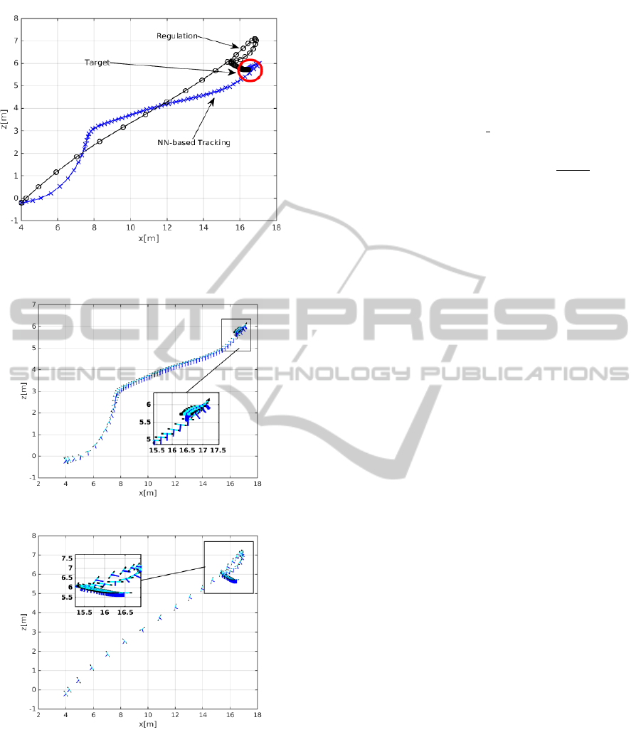
Figure 6: Comparative between the NN-based tracking and

a classical regulation control.

(a)

(b)

Figure 7: Behavior of the rotorcraft: [a] NN-bases tracking

control [b] Classical regulation.

4.1 Two-Time Scale Controller

It has been used a classical two-time scale controller

to fulﬁll the tracking objective for the translational dy-

namic subsystem (1a), where it is deﬁned a linear be-

havior through stable error polynomials u

, ˙e

) and

, ˙e

) as presented in (Sepulchre et al., 1997).

¨x = T sinθ := u

, ˙e

)

¨z = T cosθ − g := u

, ˙e

)

(11)

with u

= k

+ k

˙e

and u

= k

+ k

˙e

. Such

stable linear behavior is achieved if

T =



+ (u

+ g)



(12)

θ = θ

(t) with θ

(t) = arctan



+ g



(13)

with k

, k

and k

are positive constants. The lat-

ter assumes a time-scale separation between transla-

tion (slow dynamics) and rotational (fast dynamics)

motion. The latter assumes a time-scale separation

between translation (slow dynamics) and rotational

(fast dynamics) motion. Thus, from the error variable

θ = θ − θ

arises the following dynamics

θ = τ

−

(14)

where

is disregarded to avoid aggressive com-

mands. The controller aims to track θ

(t) while com-

pensating the torque induced by the gear, for this pur-

pose it is used the controller

= −k

− k

˙e

+ mgl sin θ (15)

5 SUMMARY AND

CONCLUSIONS

The application of self-organizing artiﬁcial neural

networks to the problem of path planning of MAV-s

have been described. It has been demonstrated that

the neural network can fuse seamlessly the informa-

tion gathered from different sensory outputs such as

vision and attitude sensors. Upon training period

comprised of carrying out pseudo-random motions,

akin birds learning how to ﬂy, the MAV can learn

landing maneuvers leading to the desired landing po-

sition. The accuracy of the landing has been found

to depend on the number of nodes used in the arti-

ﬁcial neural network as well as the training parame-

ters such as learning rate and range of activation of

the neuronal network. The resulting trajectories of

the physical model show transient errors of approxi-

mately 8 % (1 .5 m over a landing target at 18 m) and a

small overshoot of 0.7 m (4. %) required to reduce the

landing speed. Due to its low computational demand

upon completion of the ANN training, the proposed

method is likely to ﬁnd application in the develop-

ment of bio-inspired MAV-s capable of autonomous

navigation using low-cost vision and attitude sensors.

ICINCO2015-12thInternationalConferenceonInformaticsinControl,AutomationandRobotics

ACKNOWLEDGEMENTS

The authors acknowledge the support of IPSA in host-

ing one of the authors (Enikov) during his sabbatical

leave allowing the development of this collaborative

research project as well as partial support from NSF

grant # 1311851 related to the development of ANN

simulation library.

REFERENCES

(2007). Embedded control system for a four rotor UAV, vol-

ume 21.

Abbeel, P., Coates, A., Quigley, M., and Ng, A. Y. (2007).

An application of reinforcement learning to aerobatic

helicopter ﬂight. Advances in neural information pro-

cessing systems, 19:1.

Berlucchi, G. and Aglioti, S. (1997). The body in the brain:

neural bases of corporeal awareness. Trends in neuro-

sciences, 20(12):560–564.

Berthoz, A. (2000). The brain’s sense of movement. Har-

vard University Press.

Escareno, J., Rakotondrabe, M., Flores, G., and Lozano,

R. (2013). Rotorcraft mav having an onboard ma-

nipulator: Longitudinal modeling and robust control.

In Control Conference (ECC), 2013 European, pages

3258–3263. IEEE.

Fantoni, I. and Lozano, R. (2002). Nonlinear control for

underactuated mechanical systems. Springer.

Fuke, S., Ogino, M., and Asada, M. (2007). Body image

constructed from motor and tactile images with vi-

sual information. International Journal of Humanoid

Robotics, 4(02):347–364.

Gillula, J. H., Huang, H., Vitus, M. P., and Tomlin, C. J.

(2011). Design and analysis of hybrid systems, with

applications to robotic aerial vehicles. In Robotics Re-

search, pages 139–149. Springer.

Goldstein, H. (1980). Classical mechanics. Addison-

Wesley.

Graziano, M. S., Cooke, D. F., and Taylor, C. S. (2000).

Coding the location of the arm by sight. Science,

290(5497):1782–1786.

Graziano, M. S., Taylor, C. S., and Moore, T. (2002). Com-

plex movements evoked by microstimulation of pre-

central cortex. Neuron, 34(5):841–851.

Head, H. and Holmes, G. (1911). Sensory disturbances

from cerebral lesions. Brain, 34(2-3):102–254.

Hoffmann, M., Marques, H. G., Hernandez Arieta, A.,

Sumioka, H., Lungarella, M., and Pfeifer, R. (2010).

Body schema in robotics: a review. Autonomous Men-

tal Development, IEEE Transactions on, 2(4):304–

324.

Iriki, A., Tanaka, M., and Iwamura, Y. (1996). Coding of

modiﬁed body schema during tool use by macaque

postcentral neurones. Neuroreport, 7(14):2325–2330.

Kohonen, T. (1982). Self-organized formation of topolog-

ically correct feature maps. Biological cybernetics,

43(1):59–69.

Lupashin, S., Schollig, A., Sherback, M., and D’Andrea,

R. (2010). A simple learning strategy for high-speed

quadrocopter multi-ﬂips. In Robotics and Automa-

tion (ICRA), 2010 IEEE International Conference on,

pages 1642–1648. IEEE.

Martinetz, T., Schulten, K., et al. (1991). A” neural-gas”

network learns topologies. University of Illinois at

Urbana-Champaign.

Melzack, R. (1990). Phantom limbs and the concept of a

neuromatrix. Trends in neurosciences, 13(3):88–92.

Morasso, P. and Sanguineti, V. (1995). Self-organizing body

schema for motor planning. Journal of Motor Behav-

ior, 27(1):52–66.

Purwin, O. and D’Andrea, R. (2009). Performing aggres-

sive maneuvers using iterative learning control. In

Robotics and Automation, 2009. ICRA’09. IEEE In-

ternational Conference on, pages 1731–1736. IEEE.

Ramachandran, V. S. and Rogers-Ramachandran, D.

(1996). Synaesthesia in phantom limbs induced with

mirrors. Proceedings of the Royal Society of London.

Series B: Biological Sciences, 263(1369):377–386.

Sepulchre, R., Jankovic, M., and Kokotovic, P. (1997). Con-

structive Nonlinear Control. Springer-Verlag.

Stoytchev, A. (2003). Computational model for an extend-

able robot body schema.

Tsukamoto, Y. (2000). Pinpointing of an upper limb pros-

thesis. JPO: Journal of Prosthetics and Orthotics,

12(1):5–6.

ApplicationofSensoryBodySchemastoPathPlanningforMicroAirVehicles(MAVs)