Modelling and Optimization of Strictly Hierarchical Manpower System

Andrej

Skraba

, Eugene Semenkin

, Davorin Kofjaˇc

, Maria Semenkina

, Anja

Znidarˇsiˇc

Matjaˇz Maletiˇc

, Shakhnaz Akhmedova

Crtomir Rozman

and Vladimir Stanovov

Cybernetics & Decision Support Systems Laboratory, University of Maribor

Faculty of Organizational Sciences, Kidriˇceva cesta 55a, SI−4000 Kranj, Slovenia

Siberian State Aerospace University, ”Krasnoyarsky rabochy” av. 31, Krasnoyarsk, 660014, Russia

Faculty of Agriculture and Life Sciences, University of Maribor, Pivola 10, SI 2311 Hoˇce, Slovenia

Keywords:

Manpower, Supply Chain, Optimization, System Dynamics, Genetic Algorithms, Optimal Control.

Abstract:

This paper addresses the problem of the hierarchical manpower system control in the restructuring process.

The restructuring case study is described where eight topmost ranks are considered. The desired and actual

structure of the system is given by the actual numbers of men in a particular rank. The system was modelled

in the dicrete state space with state elements and ﬂows representing the recruitment, wastages and retirements.

The key issues were identiﬁed in the process as the stating of the criteria function, which are time variant

boundaries on the parameter values, the chain stucture of the system and the tendency for the system to os-

cilate at given initial conditions. The oscillatory case is presented and the dynamic programming approach

was considered in the optimization as unsuitable, examining the oscillations. The boundary space and optimal

solution space were considered by indicating the small area where the solution could be optimal. The aug-

mented ﬁnite automaton was deﬁned which was used in the optimization with the adaptive genetic algorithm.

The developed optimization method enabled us to successfully determine proper restructuring strategy for the

deﬁned manpower system.

1 INTRODUCTION

Strictly hierarchical manpower systems can be found

in many places in production, industry, the public sec-

tor and the army, for example. As a case study we will

consider the Slovenian Army, which has recenty been

under the restructuring process, where the number of

ofﬁcers in the eight topmost ranks, from Second Lieu-

tenant to Major General had to be changed according

NATO

standards (

Skulj et al., 2008;

Skraba et al.,

2011;

Skraba et al., 2015). This mean that, for exam-

ple, the nuber of men in the rank of Second Leutenant

had to be reduced from 256 down to 148; for the case

of Lieutenant, the number of men should be increased

from 258 to 289 etc. The restructuring process for the

eight topmost ranks is best described by the Figure 1.

On the x-axis of Figure 1, the eight ranks are marked

as x

. . . x

while the number of men is shown on the

x-axis. The desired values are shown by the dashed

rectangles while the actual values are shown by solid

lines. The optimal control of a large manpower sys-

tem is a challenging task (

Skraba et al., 2011;

Skraba

et al., 2015) due to the time variant boundaries of key

parameters, that determine the system (Smith, 1998;

Huang et al., 2009; Kofjaˇc et al., 2009). There have

been many atempts to provide the optimal solution

of the descibed problem such as discrete minimiza-

tion of quadratic performanceindex (Mehlman, 1980)

however, there is no proper solution provided (Taran-

tilis, 2008), which would consider the fact, that the

boundaries on the particular parameters might change

in time. For example, the recruitment policy might

be changed during the years of restructuring and the

boundaries for the recruitment parameters change ac-

cordingly. Main goal is to formulate the mathemat-

ical model of manpower system and to develop al-

gorithms, that will provide consistent, nonoscilatory

control strategies to bring the strict hierarchical man-

power system from initial states to desired end states

(Mehlman, 1980;

Skraba et al., 2011;

Skraba et al.,

2015). Since the addressed problem resembles the

supply chain, similar approaches could be applied

in e.g. inventory control, where oscillations are not

desired or in processing industry control where the

stability of the levels in chained tanks is important

(Schwartz et al., 2006).

215

Škraba A., Semenkin E., Kofjac D., Semenkina M., Znidaršic A., Maletic M., Akhmedova S., Rozman C. and Stanovov V..

Modelling and Optimization of Strictly Hierarchical Manpower System.

DOI: 10.5220/0005546002150222

In Proceedings of the 12th International Conference on Informatics in Control, Automation and Robotics (ICINCO-2015), pages 215-222

ISBN: 978-989-758-122-9

 2015 SCITEPRESS (Science and Technology Publications, Lda.)

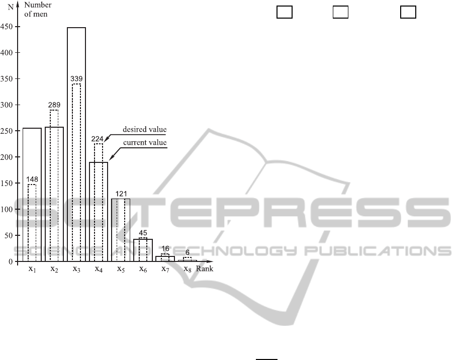
Figure 1: The desired (dashed rectangle) and actual (solid

rectangle) values in a particular rank. It can be observed,

that in the ﬁrst rank x

, the numbers should be reduced, in

increased, in x

reduced etc. This makes the control of

the chain more challenging. The initial transition process is

prone to oscillations.

2 MODELLING OF THE

MANPOWER SYSTEM

The system described could be modelled as the cas-

caded exponential delay structure with the ouﬂow in

each compartment as shown in Figure 2. Our ap-

proach differs from the well applied Markov chain

methodology (Guerry, 2014; Dimitriou and Tsantasb,

2010; Lanzarone et al., 2010) in modelling approach,

where System Dynamics (Forrester, 1973) has been

applied. In this manner, the model could be easily un-

derstood, which is important for the end users. If the

end user does not understand the model behind the so-

lution it is difﬁcult to expect, that the system will be

properly applied. The input to the system in Figure

2 is represented by u(k) where k represents the dis-

crete time step k = 0, 1, . . . . In our case, this is the

recruitment and it is the only possible input since one

could reach the topmost rank only in strict hierarchi-

cal order, from the bottom up. It is not possible, for

example, to enter the rank of Major not being the Cap-

tain ﬁrst. The modelling of the system is similar to the

u(k)

−−−−→

R(x

)

−−−−→ x

R(x

)

−−−−→ ··· x

R(x

)

−−−−→



F(x

, f

)



F(x

, f

)



F(x

, f

)

Figure 2: Cascaded Exponential Delay Structure of Man-

power System.

modelling of supply chains (Kok et al., 2005; Pastor

and Olivella, 2008; Huang et al., 2009; Chattopad-

hyay and Gupta, 2007; Feyter, 2007; Guo et al., 1999;

Kanduˇc and Rodiˇc, 2015) where similar undesired ef-

fects occur, such as bullwhip (Kok et al., 2005). Here

we consider eight ranks x

, . . . , x

, which are shown

in Figure 2. The promotions are marked with R and

are dependant on the value of the state element x

well as on the promotion parameter value r

. The

wastages are marked with F

and are also dependent

on the value of the state element x

and the value of

the ﬂuctuation coefﬁcient f

. The presented structure

is a delay chain where the change in the ﬁrst element

propagates through the whole chain. This represents

a certain difﬁculty in providing proper system control

(Aickelin et al., 2004; Bard et al., 2007; Albores and

Duncan, 2008). The system shown in Figure 2 could

be expressed by the principles of System Dynamics

(Forrester, 1973) as a the set of difference equations

in discrete form:

x(k) = x(k

) +

k−1

∑

i=k

(i) −R

out

(i)) ∆t (1)

∆x(i)

∆t

= R

(i) −R

out

(i) (2)

where Eq. 2 represents net change of state x. Stock

variables x

, x

, . . . , x

(Levels) represent the state of

the system, in our case the number of ofﬁcers in a

particular rank x

, x

, . . . , x

, while the Rate variables

R and F (both are rates) represent the change in stocks

such as transition rates R and ﬂuctuation rates F de-

ﬁned as:

• R

rate element which represents the input to the

system, i.e. recruiting, determined by value u.

• R

rate element which represents transitions from

rank x

to rank x

. R

is determined by the value

of x

and coefﬁcient r

• R

rate element which represents transitions from

rank x

to rank x

. R

is determined by the value

of x

and coefﬁcient r

, etc.

• F

rate element which represents the ﬂuctuation

from rank x

. F

is determined by the value of x

and coefﬁcient f

• F

rate element which represents the ﬂuctuation

from rank x

. F

is determined by the value of x

and coefﬁcient f

, etc.

ICINCO2015-12thInternationalConferenceonInformaticsinControl,AutomationandRobotics

216

In matrix form the system shown in Fig. 2 in discrete

space where ∆t = 1, takes the form of:

(

x(k+ 1) = Ax(k) + Bu(k)

y(k) = Cx(k) + Du(k)

(3)

where matrix A is the matrix of coefﬁcients. The in-

put u(k) to the considered system is provided by ma-

trix B to x

such that

(k+ 1) = [1−r

(k) − f

(k)] x

(k) + u(k) (4)

In our case u(k) represents the new recruitment to

rank x

which is the input of the system. The dy-

namics of the model depends on recruitment, pro-

motions and the ﬂuctuation coefﬁcients. Coefﬁcient

values r(k), f(k) and the input u(k) are determined

with regard to the historical data, approximately for

the past decade. The model was developed with

MATLAB/Simulink

(

Skraba et al., 2011;

Skraba et al.,

2015). The task to achieve the desired number of men

in particular rank is expressed as the distance to the

target function which is predeﬁned as the function

with exponential term (

Skraba et al., 2011); this dis-

tance should be minimized:

J =

∑

n=1

∑

i=0



(i) −x

(i)



∑

i=0



z(i) −x(i)



, (5)

(i) is the target function value for rank n at step

i. One should compute min

u∈U,r∈R, f∈F

J where U,

R and F are input parameters with predeﬁned value

boundaries. The deviation from the desired values is

only one part of the problem deﬁnition. As we will

see this is not sufﬁcient since there is a possibility

that oscillations in the gained strategy might occur.

Let us consider the example of three ranks, x

, x

with initial conditions x

(0), x

(0) and target

values z(k) with boundaries:

≤ u(k) ≤ UB

≤ r(k) ≤ UB

≤ f(k) ≤ UB

(6)

At each time-step the optimization problem is solved

for ψ(k+ 1):

min

u,r, f



(k) −x

(k) + f

(k)x

(k) −u(k)+

(k)r

(k)]

+ [z

(k) −x

(k) + f

(k)x

(k)−

(k)r

(k) + x

(k)r

(k)]

+ [z

(k) −x

(k)+

(k)x

(k) −x

(k)r

(k) + x

(k)r

(k)]



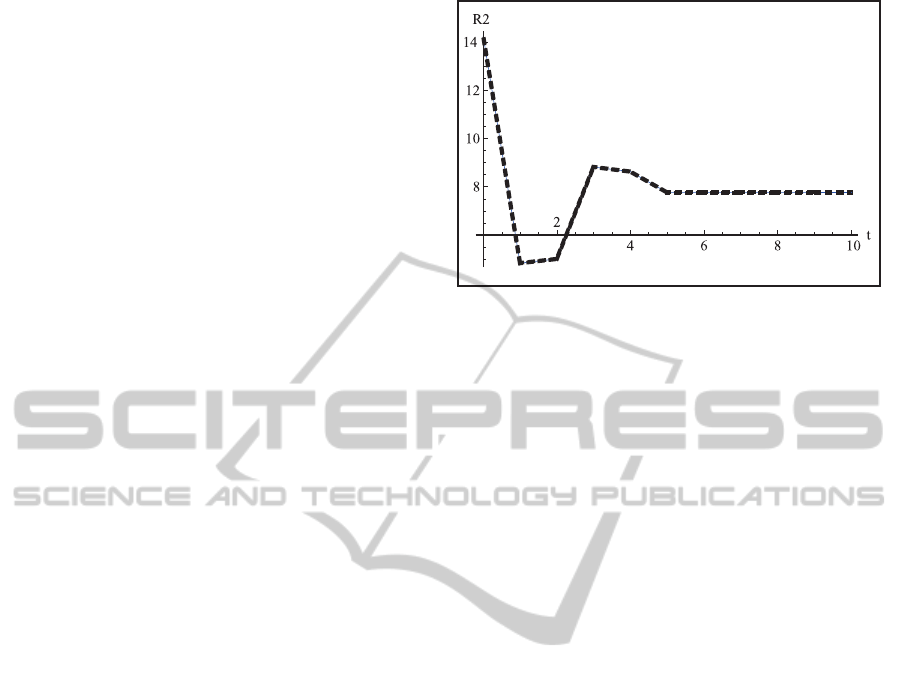
If we perform the optimization by the proposed equa-

tion the solutions might exercise undesired oscilla-

tions. Since there is no weight put on the oscillations

in the rate elements, this is possible however unde-

sired. For example, if the recruitment oscillated, it

Figure 3: Example of the oscillating promotions on the Rate

element R

would mean that one should adjust the capacity of the

training facilities accordingly which would not be de-

sired. Here one strives to get the solution in the form

of a moderate policy for all variables in question. An

example of such a solution, which is optimal if only

the distance from the desired trajectory is considered,

is shown in Figure 3. In the Figure 3 the oscilla-

tions for the promotion from the Second Lieutenant

to Lieutenant is shown. An important limitation that

should be considered when stating the optimization

problem is sensitivity to upper and lower boundaries.

If one considers only one state element with a con-

stant input for the recruitment and variable output rate

coefﬁcient, the feasability of achieving the target val-

ues is illustrated in Figure 4. On the x-axis the Lower

Boundary (LB) value is shown going from 0 to 1, sim-

ilarly for the x-axis where the Upper Boundary (UB)

is shown. On the z axis the Difference between the de-

sired and actual value is shown. Although this is only

an example, the real numbers are much higher and

such a strategy would not be acceptable. One could

observe the unfeasible region in the x-y plane due to

the lower and upper boundaries. It is interesting that

for the simplest case the optimal region in the upper

part of Figure 4 is relatively small. In this case we

actually examine the lower and upper boundary space

and observe the optimality region. As can be observed

the volume is not symmetrical leading to the possibil-

ity of searching in the direction of the lowest devia-

tion from the desired trajectory. Therefore, in order

to prevent the system from this oscillating behaviour,

the automaton A

has been constructed which consid-

ers strategies with one extremum point where:

• The set of states is S = {S

, S

}

• The comparison alphabet is A = {l, e, g}

• The initial state is i = S

• The set of terminal states is T = {S

, S

}

ModellingandOptimizationofStrictlyHierarchicalManpowerSystem

217

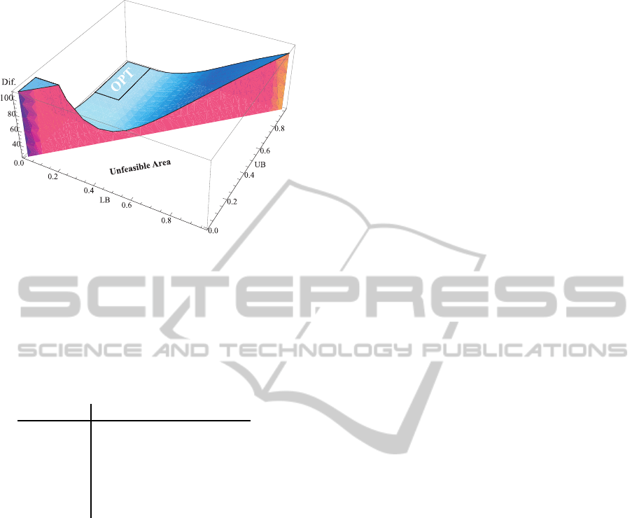
Figure 4: Feasibility region for the system with one state.

Here only the variation of the output rate element is con-

sidered. Half of the x-y plane is not feasible. The optimal

region is shown only as a small part of the parameter bound-

ary space.

• The set of probabilities in the optimization penalty

function P = {p

, p

}

The transition function of A

, δ : S×A → S is deﬁned

by the rules A:

p l e g

↔ S

← S

(7)

An important addition is the augmenting of the au-

tomaton with the probability operator p which is ap-

plied at the optimization as the penalty coefﬁcient. In

our case we can restate the criteria function as:

= min

u,r, f



A (p)

r, f,

∑

k=1



z(k) −x(k)





z(k) −x(k)

i

(8)

subject to:

min

(k) ≤ u(k) ≤ u

max

(k)

min

(k) ≤ r(k) ≤ r

max

(k)

min

(k) ≤ f(k) ≤ f

max

(k)

(9)

where A (p) represents the applied automaton with

the augmented penalty probability, which alters the

optimization function when the terminal state is not

acceptable by appropriate weight, eliminating im-

proper strategies. This is applied to the evolution-

ary algorithm and alters the value of the minimization

function when the terminal state is not acceptable ac-

cording to the appropriate weight. The automaton is

also deﬁned by the penalty coefﬁcients p

, p

and

according to the number of alternating steps that

were exercised by a particular strategy.

3 ADAPTIVE EVOLUTIONARY

ALGORITHM WITH

CONSTRAINT HANDLING

METHODS

A penalty method was developed in order to reject

the infeasible solutions which exercise oscillations of

input parameters, such as r(k) and f(k). Here, os-

cillations on the rate elements are also not desired.

The idea behind the developed penalty method is that

the discrete derivative of each r and f can be used to

see if this function changed its orientation, i.e. the

function is non-monotonic. After evaluating the er-

ror in the genetic algorithm, the feasibility is checked

at each step of the algorithm. In order to calculate

the penalty function, we have calculated the number

of times when the derivative was more than or equal

to zero, and the number of times when it was less

than zero. For each case we have also calculated the

sum of the derivative values for positive and negative

points separately. The derivative value for the input to

the system u was normalized to the interval [0,1], as

its value is much bigger than for the rest of variables

since recruitment is an absolute value and all other pa-

rameters are considered as coefﬁcients between 0 and

1. In the next step, the two conditions were checked.

Firstly, we have checked if all of the derivative values

are positive or negative. In this case, the penalty value

for this time series is zero. If there were several posi-

tive and several negative values, than the penalty size

was set to the smallest module value between the two

sums of positive and negative derivatives respectively.

The penalty calculation can be formalized as (

Skraba

et al., 2015):

penalty =







0, if (N

= T −1orN

= T −1),

|, i f S

< S

|, if S

< S

(10)

where N

and N

are the numbers of positive and neg-

ative derivative values, and S

and S

are the sums

of the positive and negative derivative values respec-

tively. These heuristic penalty values are calculated

based on the idea that if most of the time the deriva-

tive was higher than zero, than the negative values

should be changed to positive ones, so that these time

series would become feasible. The oposite action is

needed if the derivative is negative. The overall mod-

iﬁed penalty value for all the time series was Total

ICINCO2015-12thInternationalConferenceonInformaticsinControl,AutomationandRobotics

218

Penalty (TP) and used in the genetic algorithm as:

TP = C ·

k−1

∑

i=0

pnlty

∑

i=0

pnlty

+ pnlty

√

(11)

where C is a penalty weight constant and G is the cur-

rent generation number. In this case the penalty size

increases at each generation. We also used a modiﬁca-

tion of the ﬁnite automaton deﬁned as the set of rules

(7) as a constraint handling method, and its main idea

was that if the system ends up in states S

, S

or S

, it

means that the correspondingcoefﬁcient made at least

one oscillation, which is not desirable. In this case

the ﬁnite automaton returned penalty value showing

that this time series is not desirable and formed the

penalty function. The return value is shown as the p

value, deﬁned by the equation:

pnlty =











0, if p

i+1

−c

, if p

−c

i+1

, if p

i+1

−c

|+ penalty

i−1

, if p

(12)

where c

is the coefﬁcient value for the state element

i, and penalty

i−1

is the penalty value for the previous

state. The return value is zero in states S

, S

and S

For states S

and S

the return value depends on the

size of the oscillation tracked, and for the ﬁnal state

the return value was the sum of the current and

previous penalty during the oscillations of the time

series.

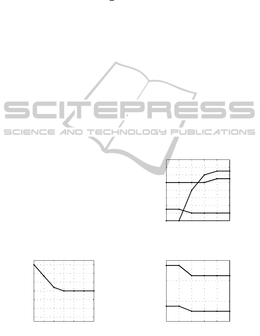
4 RESULTS

Figure 5 shows the example of the nonoscilatory dy-

namics on the state element for Second Lieutenant

(Level element L). On the x-axis the time in years

is shown. Here we consider a six year period. On the

y-axis the nunber of men in the rank of Second Leu-

tainant is shown. In this case, we have considered the

0 1 2 3 4 5 6

100

Time [year]

L [men]

Figure 5: Example of the nonoscillatory dynamics on the

state element for Second Lieutenant (Level element L).

reduction of the number of men from 100 to 70. It can

be observed that the state element does not cause os-

cillations due to the applied modiﬁed ﬁnite automaton

at the optimization process. Advanced optimization

approaches have been descibed in (Semenkin and Se-

menkina, 2012b; Semenkin and Semenkina, 2012c;

Semenkin and Semenkina, 2012a; Semenkin and Se-

menkina, 2014) with modiﬁed ﬁnite automaton (FA)

(

Skraba et al., 2014). Figure 6 shows the example

of the nonoscillatory dynamics of the promotions on

the Rate element R. Again, on the x-axis the time for

the period of six years is shown. This time, on the

y-axis, the rate of promotions is shown. The unit on

the y-axis can be noticed which is [men/year]. As one

can observe, for the case of three ﬂows, there are no

oscillations in the strategy. The system stabilizes at

time k = 5. Figure 7 shows the dynamics on the rate

elements of Fluctuations. As before, the x-axis repre-

sents time in years while the y-axis shows the rates

of ﬂuctuations with the unit of men per year. The

oscillations are not present which fulﬁls our goal of

providing a nonoscillatory strategy to achieve the de-

sired states. All three elements, state, promotion rates

as well as ﬂuctuation rates are nonoscillatory provid-

ing the moderate policy which would lead the sys-

0 1 2 3 4 5

Time [year]

R [men/year]

Figure 6: Example of the nonoscillatory dynamics of the

promotions on the Rate element R.

0 1 2 3 4 5

Time [year]

F [men/year]

Figure 7: Example of the nonoscillatory dynamics of the

ﬂuctuations F.

ModellingandOptimizationofStrictlyHierarchicalManpowerSystem

219

tem from the initial states to the desired states in the

prescribed time. Although the change might not ap-

pear to be signiﬁcant, it is obvious that the strategy

of the HQ could not examine oscillations since there

are many activities bond to one another. Besides, that

the undesired disturbances could propagate within the

whole system.

5 CONCLUSION

The determinatiion of the control strategy for the hi-

erarchical manpower system is demanding task due

to the chain structure of the considered system. The

system was sucessfully described in the discrete state

space. Another important difﬁculty is time variant

boundaries on the parameter values. The bound-

aries are also dependant on the state elements and

therefore also change in time. All the mentioned

conditions put the described problem in the ﬁeld of

hard problems

. An additional condition is that os-

cillations in any of the parameters or states are not

desirable. The approach with the classical dynamical

programming proved that oscillations are inevitable if

one only seeks the shortest time to achieve the stated

goals. By the consideration of the lower and upper

boundaries for the one state example, we have shown

that the optimal region for a particular parameter is

limited and dependent on the values of the lower and

upper boundaries. Oscillations were sucessfully ter-

minated by the application of the modiﬁed ﬁnite au-

tomaton which also considers the penalty function for

the parameter discrete derivatives. The applied adap-

tive genetic algorithm has been tested and provides

promising results for solving such complex tasks. An

important issue which was not addressed in the paper

is the user interface since the user has to deal with ap-

proximately 100 variables for controlling only eight

ranks in the period of 10 years. The develpedmethod-

ology is applicable for controlling not only the man-

power systems but also similar supply chain struc-

tures where one has to deal with the bullhip effect

(Kok et al., 2005). A general observation of the lit-

erature review showed that there is no single method

that would provide an optimum solution for the de-

scribed problem. One reason lies in the weights that

could be arbitrarily applied to a particular part of the

optimization problem.

Initially it would seem reasonable to deﬁne the

control problem only as minimization of the distance

to the target function with consideration of parameter

boundaries. Here the rationale is that the target trajec-

tory should be reached without considering the costs

when rate elements are within those prescribed, i.e.

normal boundaries. This kind of problem formula-

tion would actually yield the optimum solution if one

would like to achieve target values in the shortest pos-

sible time. An important ﬁnding is however the state-

ment of the problem, where only the minimization of

the distance to the target function by considering the

boundaries is insufﬁcient, resulting in possible unde-

sired oscillatory solutions.

An important reduction of the complexity of the

problem addressed was achieved by introducing the

Trajectory function.

In order to complete the deﬁnition of the control

problem, the acceptable strategies were described and

FA were developed accordingly. The differences be-

tween two differently stated control problems were

shown in examples. The application of FA provided

proper results where the gained strategies did not dis-

play undesired oscillation patterns. Certainly, there is

a cost that is paid for providing the proper shape of the

strategy, which was shown by the different values of

quadratic performance index, meaning that more time

is needed to achieve the desired goal.

With the application of the developed system

decision-makers were faced with considerable gaps

between desired and estimated states, which were

indicated by the results of the described scenarios.

Experts and decision-makers were certainly roughly

aware of these discrepancies, but the results provided

by the developed system offered much more explicit

and elaborated evidence of the problems related to fu-

ture trends.

The provided real world example and solution

showed that the developed approach successfully pro-

vides the strategies which could be implemented in

the real-world system. According to the stated scenar-

ios an important question concerning the attainability

of a particular rank has been answered.

An important consideration in the application of

optimization techniques is user interaction. Opti-

mization methods applied are advanced, yet the sys-

tem should enable user-friendly manipulation of input

variables. It has to be mentioned that the user inter-

face has a major role in the addressed optimization

problem. Users try to optimize the process regardless,

of advanced analytical and numerical techniques with

their knowledge about the system and previous expe-

rience. A useful user interface could solve a signif-

icant portion of the problem by a simple calculation

which is usually carried out ad hoc. The entire sys-

tem for manpower planning was developed as major

changes in the military system were made which had

not been previously faced. Drastic changes in rank

numbers yielded a new dimension to the problem of

the manpower planning of ofﬁcers who had to be sup-

ICINCO2015-12thInternationalConferenceonInformaticsinControl,AutomationandRobotics

220

ported by the new approach described here. However,

no sophisticated numerical procedure could be suc-

cessful without: a) a user friendly interface, and b) an

understanding of the problem by the user. In our case,

the target functions as well as the parameter bound-

ary values are stated as time vectors. In the worst

case, the user has to determine 43 vectors; 1 vector of

initial states, 34 boundary vectors and 8 vectors with

target trajectories in order to perform a particular op-

timization run. The minimal set of input data when

boundaries and initial states are set automatically on

the basis of historical data is the vector of goal states

with terminal time.

ACKNOWLEDGEMENT

This research is ﬁnanced by Slovenian Research

Agency ARRS, Proj. No.: BI-RU/14-15-047 and Re-

search Program Group No. P5-0018 (A).

REFERENCES

Aickelin, U., Dowsland, U., and Kathryn, A. (2004). An in-

direct genetic algorithm for a nurse-scheduling prob-

lem. Comput. Oper. Res., 31(5):761–778.

Albores, P. and Duncan, S. (2008). Government prepared-

ness: Using simulation to prepare for a terrorist attack.

Comput. Oper. Res., 35(6):1924–1943.

Bard, J. F., Morton, D., and Wang, Y. (2007). Workforce

planning at USPS mail processing and distribution

centers using stochastic optimization. Ann. Oper. Res.,

2007(155):51–78.

Chattopadhyay, A. K. and Gupta, A. (2007). A stochastic

manpower planning model under varying class sizes.

Ann. Oper. Res., 2007(155):41–49.

Dimitriou, V. A. and Tsantasb, N. (2010). Evolution of a

time dependent markov model for training and recruit-

ment decisions in manpower planning. Linear Algebra

and its Applications, 433(11-12):1950–1972.

Feyter, T. D. (2007). Modeling mixed push and pull pro-

motion ﬂows in manpower planning. Ann. Oper. Res.,

2007(155):25–39.

Forrester, J. (1973). Industrial Dynamics. MIT Press, Cam-

bridge, MA.

Guerry, M.-A. (2014). Some results on the embeddable

problem for discrete-time markov models in man-

power planning. Communications in Statistics - The-

ory and Methods, 43(7):1575–1584.

Guo, Y., Pan, D., and Zheng, L. (1999). Modeling mixed

push and pull promotion ﬂow. Ann. Oper. Res.,

1999(87):191–198.

Huang, H.-C., Lee, L.-H., Song, H., and Thomas Eck, B.

(2009). Simman-a simulation model for workforce

capacity planning. Comput. Oper. Res., 36(8):2490–

2497.

Kanduˇc, T. and Rodiˇc, B. (2015). Optimization of a fur-

niture factory layout. Croatian Operational Research

Review, 6(1):121–130.

Kofjaˇc, D., Kljaji´c, M., and Rejec, V. (2009). The anticipa-

tive concept in warehouse optimization using simula-

tion in an uncertain environment. European Journal

of Operational Research, 193(3):660–669.

Kok, T., Janssen, F., Doremalen, J., Wachem, E., Clerkx,

M., and Peeters, W. (2005). Philips electronics syn-

chronizes its supply chain to end the bullwhip effect.

Interfaces, 35(1):37–48.

Lanzarone, E., Matta, A., and Scaccabarozzi, G. (2010).

A patient stochastic model to support human resource

planning in home care. Production Planning & Con-

trol, 21(1):3–25.

Mehlman, A. (1980). An approach to optimal recruitment

and transition strategies for manpower systems using

dynamic programming. Journal of Operational Re-

search Society, 31:1009–1015.

Pastor, R. and Olivella, J. (2008). Selecting and adapting

weekly work schedules with working time accounts:

A case of a retail clothing chain. European Journal of

Operational Research, 184:1–12.

Schwartz, J. D., Wang, W., and Rivera, D. E. (2006).

Simulation-based optimization of process control

policies for inventory management in supply chains.

Automatica, 42(8):1311–1320.

Semenkin, E. and Semenkina, M. (2012a). The choice

of spacecrafts’ control systems effective variants with

self-conﬁguring genetic algorithm. In Informatics in

Control, Automation and Robotics: Proceedings of

the 9th International Conference ICINCO, pages 84–

93.

Semenkin, E. and Semenkina, M. (2012b). Self-conﬁguring

genetic algorithm with modiﬁed uniform crossover

operator. In Tan, Y., Shi, Y., and Ji, Z., editors, Ad-

vances in Swarm Intelligence, volume 7331 of Lecture

Notes in Computer Science, pages 414–421. Springer

Berlin Heidelberg.

Semenkin, E. and Semenkina, M. (2012c). Self-

conﬁguring genetic programming algorithm with

modiﬁed uniform crossover. In Proceedings of the

Congress on Evolutionary Computations of the IEEE

World Congress on Computational Intelligence (CEC

WCCI 2012), pages 1918–1923, Brisbane, Australia.

SCITEPRESS.

Semenkin, E. and Semenkina, M. (2014). Stochastic mod-

els and optimization algorithms for decision support

in spacecraft control systems preliminary design. In

Ferrier, J.-L., Bernard, A., Gusikhin, O., and Madani,

K., editors, Informatics in Control, Automation and

Robotics, volume 283 of Lecture Notes in Electri-

cal Engineering, pages 51–65. Springer International

Publishing.

Skraba, A., Kofjaˇc, D.,

Znidarˇsiˇc, A., Maletiˇc, M., Rozman,

C., Semenkin, E. S., Semenkina, M. E., and Stanovov,

V. V. (2015). Application of self-gonﬁguring genetic

algorithm for human resource management. ournal of

Siberian Federal University. Mathematics & Physics,

8(1):94–103.

ModellingandOptimizationofStrictlyHierarchicalManpowerSystem

221

Smith, J. (1998). The Book. The publishing company, Lon-

don, 2nd edition.

Tarantilis, C. (2008). Editorial: Topics in real-time sup-

ply chain management. Computers & Operations Re-

search, 2008(35):3393–3396.

Skraba, A., Kljaji´c, M., Papler, P., Kofjaˇc, D., and Obed, M.

(2011). Determination of recruitment and transition

strategies. Kybernetes, 40(9/10):1503–1522.

Skraba, A., Semenkin, E., Semenkina, M., Kofjaˇc, D.,

Znidarˇsiˇc, A.,

C. Rozman, Maletiˇc, M., Akhmedova,

S., and V.Stanovov (2014). Development of discrete

manpower model and determination of optimal con-

trol strategies. In Proceedings of the XVIII Inter-

national Scientiﬁc Conference Reshetnev Readings,

pages 421–423, Krasnoyarsk, Russia. SibSAU.

Skulj, D., Vehovar, V., and

Stamfelj, D. (2008). The

modelling of manpower by Markov chains - a case

study of the Slovenian armed forces. Informatica,

2008(32):289–291.

ICINCO2015-12thInternationalConferenceonInformaticsinControl,AutomationandRobotics

222