Identifying Landmark Cues with LIDAR Laser Scanner Data Taken

from Multiple Viewpoints

Andrzej Bieszczad

California State University Channel Islands, One University Drive, Camarillo, CA 93012, U.S.A.

Keywords: Robot, Navigation, Localization, Cue Identification, Neural Networks, Support Vector Machines,

Classification, Pattern Recognition.

Abstract: In this paper, we report on our ongoing efforts to build a cue identifier for mobile robot navigation using a

simple one-plane LIDAR laser scanner and machine learning techniques. We used simulated scans of

environmental cues to which we applied various levels of Gaussian distortion to test a number of models the

effectiveness of training and the response to noise in input data. We concluded that in contrast to back

propagation neural networks, SVM-based models are very well suited for classifying cues, even with

substantial Gaussian noise, while still preserving efficiency of training even with relatively large data sets.

Unfortunately, models trained with data representing just one stationary point of view of a cue are inaccurate

when tested on data representing different points of view of the cue. Although the models are resilient to noisy

data coming from the vicinity of the original point of view used in training, data that originates in a point of

view shifted forward or backward (as would be the case with a mobile robot) proved much more difficult to

classify correctly. In the research reported here, we used an expanded set of synthetic training data

representing three view points corresponding to three positions in robot movement in relation to the location

of the cues. We show that by using the expanded data the accuracy of cue classification is dramatically

increased for test data coming from any of the points.

1 INTRODUCTION

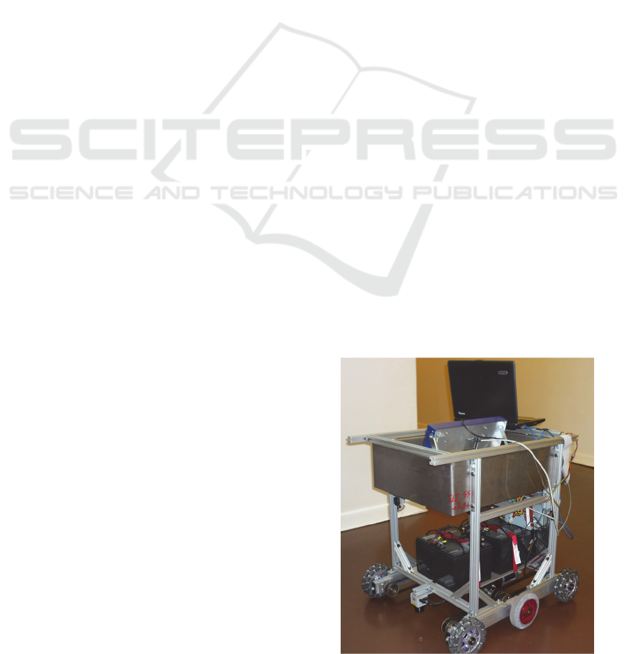
Automated Intelligent Delivery Robot (AIDer; shown

in Figure 1) is a mobile robot platform for exploring

autonomous intramural office delivery (Hilde et al.,

2009; Rodrigues et al., 2009). The research reported

in this paper was part of the overall effort to explore

ways to deliver such functionality. The robot was to

navigate in a known environment (a map of the

facility is one of the elements of AIDer’s

configuration) and carry out tasks that were requested

by the users through a Web-based application. Each

request included the location of a load that was to be

moved to another place that was also specified in the

request. The pairs of start and target locations were

entered into a queue that was managed by a path

planning module. When the next job from the queue

was selected, the robot was directed first to the start

location where it was to get loaded after announcing

itself, and then to the destination where it was to get

unloaded after announcing its arrival. That routine

was to be repeated indefinitely — if there were other

requests waiting in the queue and as long as there was

power.

Figure 1: Robot with a laser scanner (between the front

wheels).

Bieszczad A..

Identifying Landmark Cues with LIDAR Laser Scanner Data Taken from Multiple Viewpoints.

DOI: 10.5220/0005508000780085

In Proceedings of the 12th International Conference on Informatics in Control, Automation and Robotics (ICINCO-2015), pages 78-85

ISBN: 978-989-758-122-9

 2015 SCITEPRESS (Science and Technology Publications, Lda.)

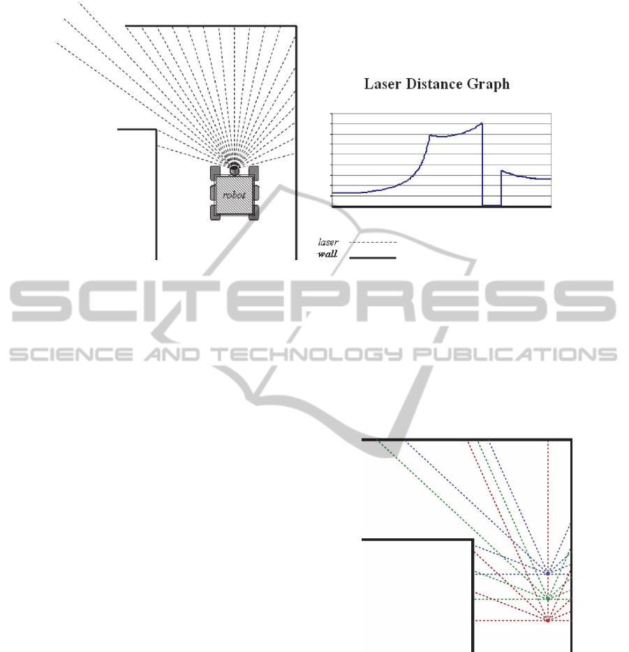
Figure 2: Robot LIDAR scan and the corresponding graph.

One of the major objectives was to provide the

functionality at low cost. Therefore, AIDer has a very

limited set of sensors for navigation: right side

detectors of the distance from the wall, and a frontal

2D (one-plane) LIDAR laser scanner for detecting

cues such as turns and intersections. The side sensors

are used to provide a real-time feedback to a

controller that corrects the position of the robot so it

stays at a constant distance from the right wall (Hilde

et al., 2007).

Higher-level navigation in AIDer is based on

following paths that consist of a series of intervals

between landmarks (Rodrigues et al., 2009). A map

of the facility is provided as an element of the

configuration (using a custom notation), so the robot

is not tasked with mapping the environment. The map

configuration file includes locations of landmarks

along with exact distances between the landmarks.

Upon receiving the next task to carry out, the robot

determines the path to travel in terms of the

landmarks. The path is divided into a sequence of

landmarks, and the robot is successively directed to

move to the next landmark. After the current target

landmark is identified, the robot receives the next

target landmark to go to. To accommodate for error

in mobility (like slippage of the wheels) that may

skew the robot orientation based purely on traveling

exact distances, the robot relies on identification of

cues to verify reaching landmarks.

In an environment lacking GPS, identification of

environmental cues is a critical low-level task

necessary for recognizing landmarks (Thrun, 1998),

since landmarks are defined in terms of cues. The

frontal laser-scanner in AIDer serves that purpose.

Each scan produces a sequence of measurements that

differ depending on the shape of the surrounding

walls. For example, Figure 2 shows a scan of a left

turn. The scan results - a sequence of numbers

representing the measured distance (e.g., in inches) -

are graphed using angles on the x axis and the

distances on the y axis. Due to the range limitations

of the laser scanner, certain measurement may be read

as zeros; that is visible as a sudden drop in the curve

shown in the figure.

Figure 3: Multipoint view of a cue “left turn”. Only 9

measurements from each viewpoint shown here for clarity.

In (Hilde et al., 2007), an approach similar to

(Hinkel et al, 1988) was taken with a selective subset

of measurements used to define cues analytically with

a limited success.

In this paper, the complete raw set is used for this

purpose as will be shortly explained. Our earlier

attempts to use raw data in such a way were not

completely successful (Henderson, 2012), and the

research reported here remedies that.

IdentifyingLandmarkCueswithLIDARLaserScannerDataTakenfromMultipleViewpoints

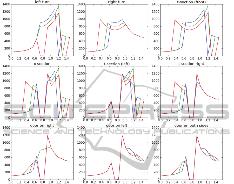
Figure 4: Three curves corresponding to three points of view for each of the nine cues. The y axis shows LIDAR measurements

given in inches, and the x axis shows progression of the angle for each successive measurement.

2 RELATED WORK

Mapping and localization services are the foundation

of autonomous navigation (Thrun, 1998). As we

already stated, mapping is not a functional objective

of the AIDer. Vast majority of the current localization

work is based on utilization of very sophisticated

equipment as seen in cars participating in R&D

efforts in academia, auto industry, and government-

sponsored contests (e.g., Leonard et al., 2008).

Utilizing simple sensors with very limited capabilities

started the field (Borenstein, 1997), but currently it’s

rare to depend on just such limited functionality. Yet,

the use of inexpensive devices is important in

environments lacking access to powerful computers

or abundant power supplies (e.g., Roman et al., 2007),

and when cost is a concern (e.g., Tan et al., 2010).

LIDAR-based identification was successfully

solved by analytical methods in (Hinkel et al, 1988)

in which histograms of laser measurements were used

as the input data. There have been numerous attempts

to use similar data using a variety of analytical

approaches (e.g., Zhang et al., 2000; Shu et al., 2013;

Kubota et al., 2007; Nunez et al., 2006).

(Vilasis-Cardona et al., 2002) used cellular neural

networks to classify cues, but the localization was

based on processing 2D images of vertical and

horizontal lines placed on the floor rather then 1D

LIDAR measurements. Just like in (Henderson,

2012), histogram data were used as inputs to

backpropagation neural network in research reported

in (Harb et al., 2010), but the authors did not specify

the details of the back propagation algorithm that they

used. In (Bieszczad, 2015), we follow that sub

symbolic approach studying the capabilities of back

propagation models and contrasting them with

training based on support vector machines (SVM).

ICINCO2015-12thInternationalConferenceonInformaticsinControl,AutomationandRobotics

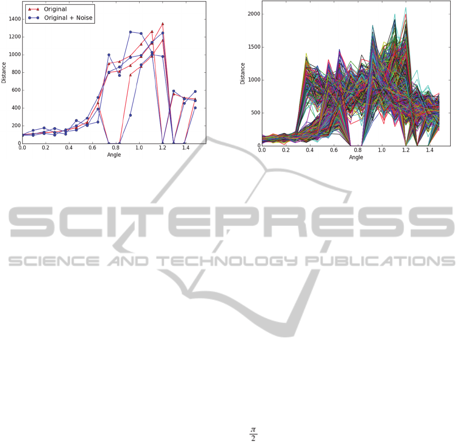
Figure 5: Three cue curves corresponding to three different

points of view of the cue lt along with their distorted

versions obtained by applying Gaussian noise

 = 0.2. All of these curves must classify as lt.

3 CUE DATA SETS

3.1 Single-point View

The laser mounted on AIDer is capable of scanning

180o with a granularity yielding 512 measurements

per scan. Such a high-dimension space would be

inconvenient for exploration of the techniques, so in

(Bieszczad, 2015) we handcrafted a smaller,

17dimensional, synthetic data set for a miniaturized

virtual model that otherwise preserved the geometry

of the office environment and the nature of the

problem. Our results reported in (Bieszczad, 2015)

indicated that good models can be built with both

back-propagation neural networks applying

Broyden–Fletcher–Goldfarb–Shannon (BFGS)

optimization augmented with regularization, and with

Support Vector Machines (SVM) assuming that data

shaping took place with a normalization followed by

Principal Component Analysis (PCA). Neural

networks using another optimization approaches

were not as successful frequently failing to converge

and yielding large errors.

Unfortunately, we also showed that expanding

data dimension thirty-fold, from 17 back to the

original 512-dimensional space was not handled well

by the models built using neural network techniques.

Training was failing or taking too long to converge on

a relatively fast platform that we had available for the

experiments (see TABLE 1 and 2).

In contrast to the models built with neural

networks, SVM models overcame the challenges and

scaled up very well preserving the effectiveness of

training and the accuracy of classification.

Figure 6: One thousand curves representing randomly

generated cues with applied noise with  = 0.2.

3.2 Multi-point View

In the research reported in this paper, we use the same

approach, namely training an SVM (Bieszczad,

2015), but with the original problem expanded from

identifying a cue from a single point of view to

identifying cues from multiple, namely three, points

of view.

Following the same illustrative approach shown

in Figure 2, if we take LIDAR snapshots from three

points as shown in Figure 3, then we obtain three

model curves for each of the original nine cues: lt (left

turn), rt (right turn), ts (t-section/front), xs (x-section),

tl (left t-section), tr (right t-section), dr (door on

right), dl (door on left), and d2 (door on both sides).

In this miniaturized model (rather than the original

model with 512 dimensions) every (simulated) scan

is a sequence of distance measurements made with

the laser angle progressing in 17 steps in the interval

[0, ]. All curves are shown in Figure 4.

As in the earlier experiments we apply Gaussian

noise to all curves for training and for testing. Figure

5 illustrates the level of distortion of three curves

corresponding to the cue lt caused by applying noise

with a standard deviation =0.2. Both the

normalization and the PCA transforms are built using

only the training data, and then applied to test data.

The data present a very challenging task for

classifiers as illustrated in Figure 6; the curves

representing the cues are similar in many respects.

The PCA analysis of the cue data shows that although

the clusters are noticeable, they are overlapping as

shown in Figure 7.

We attempted to apply dimension reduction using

PCA, but that led to increased error rates; especially

with larger noise. Indeed, even with the low

dimensional cue data a closer examination of the

IdentifyingLandmarkCueswithLIDARLaserScannerDataTakenfromMultipleViewpoints

principal components revealed that most of the

dimensions were actually significant as shown by

computing the variance ratios:

[ 0.27065951 0.19814385 0.13178777

0.05885712 0.04639313 0.03896735

0.03728837 0.03559292 0.03151982

0.02958179 0.02692341 0.0266508

0.02205014 0.02059795 0.01286112

0.00689689 0.00522805]

4 RESULTS

4.1 Testing One-viewpoint Model

Our first fundamental question was if the model

trained with data generated from one point of view

(the midpoint in Figure 3) can identify same cues as

perceived from different points of view (backward

and forward; shifted by a delta that is the same as the

distance from the wall in our data set). We generated

training samples just like we did in (Bieszczad, 2015):

we applied Gaussian noise to distort the curves

corresponding to cues taken from the midpoint to

generate ten thousand samples. An SVM model built

promptly on our computing platform, so we could test

a number of variants. However, unlike in (Bieszczad,

2015) this time around we generated test sets from

curves corresponding to measurements taken from all

three (rather than just one) points.

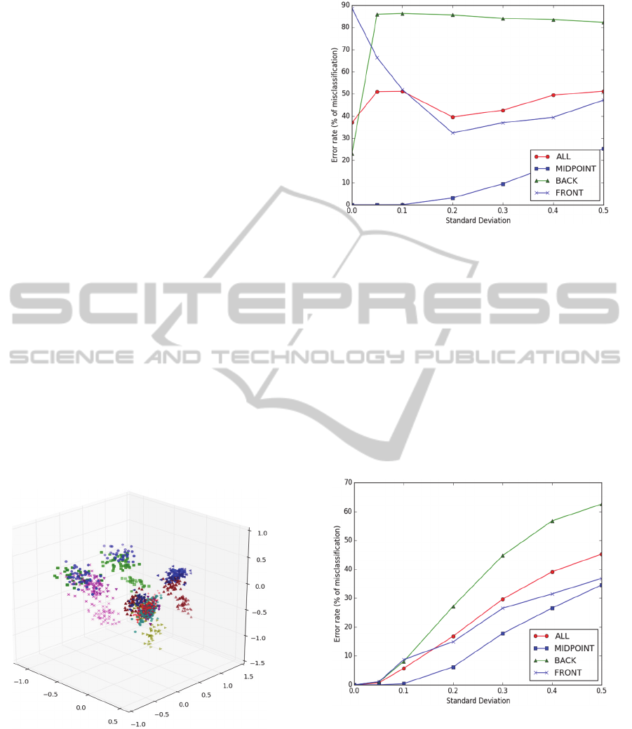
Figure 7: Clusters obtained with the principal component

analysis applied to one thousand curves representing

randomly generated cues with applied noise with  = 0.2.

Please note that for drawing in 3D only the first three

principal components are used. Although the clusters are

overlapping in 3D, they are much better separated in higher

dimensions.

Figure 8: Performance of the SVM model created using a

training set generated from cue curves taken from a single

point of view, but test against test sets created from all and

from each individual point of view.

We applied random noise to randomly selected

ten thousand of test samples and then tested the set

against a number of models built with different levels

of distortion (i.e., noise). As shown in Figure 8, the

model preserves the accuracy of the curves

concentrated around the viewpoint used for

generating training set, but fails badly for curves that

represent cues from different point of views. It also

performs poorly if the test set is constructed randomly

using cue scans taken from all points of view.

Figure 9: Performance of the SVM model created using a

training set generated from cue curves taken from a

multiple points of view, and tested against test sets created

from all and from each individual point of view.

4.2 Testing Multi-view Model

In an attempt to find a remedy, we created a model

using our extended data set generated as described

ICINCO2015-12thInternationalConferenceonInformaticsinControl,AutomationandRobotics

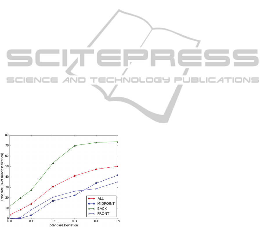
earlier from three different points of view. We tested

the model in the same way as the former.

The results can be seen in Figure 9. Comparing

the graphs with the ones drawn in Figure 8 shows that

the new model performs dramatically better on all test

data sets although not as well as the single-point

model performed with the test data taken from the

same single point of view that was used for training.

Still, the identification of cues scanned from the mid-

point is very close to the one shown in Figure 8,

although the impact of high-level of distortion on the

error rate is stronger. As before, the scans from the

back point of view are most difficult to identify, but

evidently moving the robot forward is less of the

problem in this particular environment.

5 CONCLUSIONS

We showed that the cue identification model first

presented in (Henderson, 2012) and (Bieszczad,

2015) can be improved by extending the training set

to data collected from multiple points of view. Such a

model will be more accurate for the robot in motion.

Therefore, the need to pinpoint exactly the location

most appropriate to take a scan for identification is

somewhat relaxed. Instead of a single point of

opportunity, now the robot has a window of

opportunity to identify cues.

Figure 10: Performance of the SVM model created using

data with dimension reduced to three principal components.

We tried to reduce the dimension of the data used

in our experiments by trimming them down to just

three principal components. Unfortunately, as in our

earlier experiments we did end up with models that

were performing substantially worse than the models

preserving the original dimensionality of data as

illustrated by the results shown in Figure 10.

These results indicate that a machine learning

approach is a viable alternative to analytical methods

originating in (Hinkel et al., 1998), although more

experiments are needed that will test the method with

a higher granularity of robot movements (e.g.,

continuous movement) and well as robot orientation.

6 FUTURE DIRECTIONS

Using a physical machine for numerous experiments

is inconvenient and inefficient, so we are planning to

build a simulator with which it would be easier to test

our models. Such a simulator will also help us in

using a better granularity for multiple view points.

Instead of just three points, we will be able to select a

range of robot displacements (up to continuous) and

work with scans from within that range. The

capability to generate such improved data sets will be

useful in both testing our current models and in

building potentially improved models.

One important problem set aside in this paper is

the fact that cues often are present together at the

same time, so scans may include data for multiple

cues. In the current approach, such a complex super-

cue is just another cue. However, decomposing

complex cues may be a viable alternative; especially

in a more diversified environment and if a 360°

scanner is used — as we plan. We plan to use data

sets that mix cues to some degree to test the

identification capabilities of the models trained under

such circumstances. One idea to deal with this

problem — if it arises — is to extract individual cues

from curves. Such attempts have been made by some

researchers in the papers listed in the references (e.g.,

Vilasis-Cardona, 2002), and in more complex

approaches to the localization problem (e.g., through

feature extraction using image processing

techniques).

A difficult problem to overcome is the issue of

accuracy of laser scans when dealing with light

conditions and various materials from which

obstacles are made. These issues are of paramount

importance in outdoor navigation in an unknown

terrain as described in (Roman et al., 2007) and

elsewhere. To explore possible solutions — and in

general to test in in the physical world the ideas

explored with the simulator — we are in a process of

building a smaller robot similar to AIDer that is both

more convenient to use, and substantially less

expensive.

Another venue that we are planning to explore is

acquiring goal-oriented behavior based on our earlier

work on Neurosolver (Bieszczad, 1996).

IdentifyingLandmarkCueswithLIDARLaserScannerDataTakenfromMultipleViewpoints

Table 1: Software Environment.

Software Version

Python

3.4.2 64bit [GCC 4.2.1 Compatible Apple

LLVM 6.0 (clang-600.0.54)]

IPython 2.3.1

OS Darwin 14.1.0 x86_64 i386 64bit

numpy 1.9.1

scipy 0.15.1

matplotlib 1.4.2

sklearn 0.15.2

neurolab 0.3.5

Table 2: Hardware Environment.

System iMac Retina 5K, 27-inch, Late 2014

Processor 4 GHz Intel Core 7 (4 cores)

Memory 32 GB 1600 MHz DDR3

ACKNOWLEDGEMENTS

We would like to thank Advanced Motion Control

(AMC), a Camarillo, CA, company that generously

made their AIDer robot available to us.

REFERENCES

Hilde, L., 2009. Control Software for the Autonomous

Interoffice Delivery Robot. Master Thesis, Channel

Islands, California State University, Camarillo, CA.

Rodrigues, D., 2009. Autonomous Interoffice Delivery

Robot (AIDeR) Software Development of the Control

Task. Master Thesis, Channel Island, California State

University, Camarillo, CA.

Thrun, S., 1998. Learning metric-topological maps for

indoor mobile robot navigation. In Artificial

Intelligence, Vol. 99, No. 1, pp. 21-71.

Hinkel, R, and Knieriemen, T., 1988. Environment

Perception with a Laser Radar in a Fast Moving Robot.

In Robot Control 1988 (SYROCO'88): Selected Papers

from the 2nd IFAC Symposium, Karlsruhe, FRG.

Henderson, A. M., 1012. Autonomous Interoffice Delivery

Robot (AIDeR) Environmental Cue Detection. Master

Thesis, Channel Island, California State University,

Camarillo, CA.

Leonard, J., How, J., Teller, S., Berger, M., Campbell, S.,

Fiore, G., Fletcher, L., Frazzoli, E., Huang, A.,

Karaman, S., Koch, O., Kuwata, Y., Moore, D., Olson,

E., Peters, S., Teo, J., Truax, R., Walter, M., Barrett, D.,

Epstein, A., Maheloni, K., Moyer, K., Jones, T.,

Buckley, R., Antone, M., Galejs, R., Krishnamurthy, S.,

and Williams, J., 2008. A Perception-Driven

Autonomous Urban Vehicle. In Journal of Field

Robotics, 1–48.

Borenstein, J., Everett, H.R. , Feng, L., and Wehe, D., 1997,

Mobile Robot Positioning: Sensors and Techniques.

Invited paper for the Journal of Robotic Systems,

Special Issue on Mobile Robots. Vol. 14, No. 4, April

1997, pp. 231-249.

Tan, F., Yang, J., Huang, J., Jia, T., Chen, W. and Wang, J.,

2010. A Navigation System for Family Indoor Monitor

Mobile Robot. In The 2010 IEEE/RSJ International

Conference on Intelligent Robots and Systems, October

18-22, 2010, Taipei, Taiwan.

Roman, M., Miller, D., and White, Z., 2007. Roving Faster

Farther Cheaper. In 6th International Conference on

Field and Service Robotics - FSR 2007, Jul 2007,

Chamonix, France. Springer, 42, Springer Tracts in

Advanced Robotics; Field and Service Robotics.

Vilasis-Cardona, X., Luengo, S., Solsona, J., Maraschini,

A., Apicella, G. and Balsi, M., 2002. Guiding a mobile

robot with cellular neural networks. In

INTERNATIONAL JOURNAL OF CIRCUIT THEORY

AND APPLICATIONS Int. J. Circ. Theor. Appl. 2002;

30:611–624.

Shu, L., Xu, H., and Huang, M., 2013. High-speed and

accurate laser scan matching using classified features”.

In 2013 IEEE International Symposium on Robotic and

Sensors Environments (ROSE), 2013 , Page(s): 61 - 66.

Nunez, P. Vazquez-Martin, R. del Toro, J. C. Bandera, A.

and Sandoval, F., 2006. Feature extraction from laser

scan data based on curvature estimation for mobile

robotics. In Robotics and Automation (ICRA), 2006

IEEE International Conference on. IEEE, 2006, pp.

1167–1172.

Zhang, L. and Ghosh, B. K., 2000. Line segment based map

building and localization using 2d laser rangefinder. In

Robotics and Automation (ICRA), 2000 IEEE

International Conference on Robotics8 Automation,

vol. 3. IEEE, 2000, pp. 2538–2543.

Harbl M., Abielmona, R., Naji, K.,and Petriu, E., 2010.

Neural Networks for Environmental Recognition and

Navigation of a Mobile Robot. In Proceedings of IEEE

International Instrumentation and Measurement

Technology Conference, Victoria, Vancouver Island,

Canada.

Kubota, S., Ando, Y., and Mizukawa, M., 2007. Navigation

of the Autonomous Mobile Robot Using Laser Range

Finder Based on the Non Quantity Map. In

International Conference on Control, Automation and

Systems, COEX, Seoul, Korea.

ICINCO2015-12thInternationalConferenceonInformaticsinControl,AutomationandRobotics

Bieszczad, A., 2015. Identifying Robot Navigation Cues

with a Simple LIDAR Laser Scanner. Submitted to

International Workshop on Artificial Neural Networks

and Intelligent Information Processing ANNIIP 2015.

Bieszczad, A. and Pagurek, B. (1998), Neurosolver:

Neuromorphic General Problem Solver. In Information

Sciences: An International Journal 105 (1998), pp.

239-277, Elsevier North-Holland, New York, NY.

IdentifyingLandmarkCueswithLIDARLaserScannerDataTakenfromMultipleViewpoints