A Discretization Method for the Detection of Local Extrema and

Trends in Non-discrete Time Series

Konstantinos F. Xylogiannopoulos

, Panagiotis Karampelas

and Reda Alhajj

Department of Computer Science, University of Calgary, Calgary, Alberta, Canada

Department of Informatics and Computers, Hellenic Air Force Academy, Dekelia Air Base, Athens, Greece

Keywords: Moving Linear Regression Angle, Linear Regression, Pattern Detection, Trend Detection, Local Extrema,

Local Minimum, Local Maximum, Discretization.

Abstract: Mining, analysis and trend detection in time series is a very important problem for forecasting purposes. Many

researchers have developed different methodologies applying techniques from different fields of science in

order to perform such analysis. In this paper, we propose a new discretization method that allows the detection

of local extrema and trends inside time series. The method uses sliding linear regression of specific time

intervals to produce a new time series from the angle of each regression line. The new time series produced

allows the detection of local extrema and trends in the original time series. We have conducted several exper-

iments on financial time series in order to discover trends as well as pattern and periodicity detection to fore-

cast future behavior of Dow Jones Industrial Average 30 Index.

1 INTRODUCTION

The study of time series is a very important research

area for many different applications and scientific do-

mains. Any variable that changes over time can be de-

fined as a time series. The study of such variables and

their change over time can be very important for var-

ious reasons, e.g., to understand past behavior and

based on that predict future behavior. Such studies are

very important since they can be applied to a wide

spectrum of scientific fields such as psychology, eco-

nomics, physics, meteorology, geology, biology, etc.

Usually, a variable and its representation as a time

series involve real values. Therefore, a direct analysis

over these values can be extremely difficult since, for

example, if we want to analyze temperatures in Can-

ada the values may vary from -50 degrees Celsius up

to 40 degrees Celsius. Having also one decimal digit

for every observation it means that we have 901 dis-

crete values to be analyzed. Due to this wide range of

values in order to proceed with their analysis, a dis-

cretization of the time series must first be conducted.

For this purpose, many discretization techniques have

been developed (Yang et al. 2005). Discretization

groups values that are close (the closeness depends on

the discretization method and its parameters), and

then the new time series can be analyzed, e.g., detect-

ing patterns that occur often. For the discretization, a

predefined alphabet is used and a specific letter from

the alphabet is assigned to each group of data values.

By applying this method continuous (real) values can

be transformed to discrete values and, therefore, pat-

tern, periodicity or trend detection can be performed.

In this paper, we present a new discretization

method that allows us to directly identify local min-

ima/maxima and trends inside a time series. By ap-

plying a mathematical transformation on the original

time series’ values we use the outcome to perform

sliding linear regression analysis of short time inter-

vals. We have named this method Moving Linear Re-

gression Angle (MLRA) because for each linear re-

gression analysis we use the angle of the regression

line (calculated from its slope) in order to create a new

time series. Using this new time series we can detect

fast the turning points of the time series, i.e., the local

minima and maxima. Having such information we

can detect all sub-trends that exist in a time series

since the discretization method uses the same alpha-

bet letter for up or down trends. The conducted testing

demonstrates the applicability and effectiveness of

the proposed approach.

The rest of the paper is organized as follows: Sec-

tion 2 is a review of discretization and trend detection

methods. Section 3 presents the proposed MLRA

based approach. Section 4 reports the experimental

results obtained using financial data and more

346

Xylogiannopoulos K., Karampelas P. and Alhajj R..

Discretization Method for the Detection of Local Extrema and Trends in Non-discrete Time Series.

DOI: 10.5220/0005401203460352

In Proceedings of the 17th International Conference on Enterprise Information Systems (ICEIS-2015), pages 346-352

ISBN: 978-989-758-096-3

 2015 SCITEPRESS (Science and Technology Publications, Lda.)

specifically Dow Jones Industrial Average 30 Index.

Section 5 is conclusions and future work.

2 RELATED WORK

Due to the importance of analyzing time series and

especially those produced by continuous values,

many different discretization methods have been de-

veloped so far. Variables can be categorized as quali-

tative or quantitative (Yang et al. 2005). Each cate-

gory can be sub-categorized to nominal and ordinal

for qualitative and to interval or ratio for quantitative

variables. We study the second category of quantita-

tive data because of its importance and wide spectrum

of applications in various scientific domains. Differ-

ent taxonomies can be applied for the discretization

of quantitative values such as univariate or multivar-

iate, disjoint or non-disjoint, ordinal or nominal fuzzy

or non-fuzzy, etc. (Yang et al. 2005) Some of the most

common discretization methods are (a) equal-width

where each range has the same width, (b) equal-fre-

quency where the data are classified to ranges that

have the same amount of data, (c) clustered-based by

grouping data values together based on specific parti-

tions, (d) fuzzy discretization which applies its rules

based on a membership function, etc. (Bao, 2008)

Many methods have been introduced in the past

decades for forecasting purposes based on historical

data of a given time series. Esling and Agon (2012)

summarized many data mining techniques for the

analysis of time series, while White and Granger

(2011) provided a deep analysis of trends in financial

time series. Especially in finance some of the methods

can be classified as (a) numerical linear models like

ARIMA (Bao, 2008; Bao et al., 2013; De Gooijer and

Hundman, 2006; Kovalerchuck and Vityaev, 2000;

Qin and Bai, 2009; Xi-Tao, 2006), (b) rule-based

models like decision tree, naïve Bayesian classifier,

hidden Markov model etc. (Bao, 2008; Kovalerchuck

and Vityaev, 2000 ), non-linear models such as artifi-

cial networks (Balkin and Ord, 2000; Bao et al., 2013;

Qin and Bai, 2009; Selvarantnam and Kirley, 2006)

and (d) fuzzy system models and support vector ma-

chines (Muller et al., 1997; Qin and Bai, 2009).

Moreover, more financial forecasting tools have

been introduced for over a century based on technical

analysis. Such methods are Moving Average for dif-

ferent time spans, Relative Strength Index, Moving

Average Convergence Divergence for different time

spans, Momentum, etc. (Bao, 2008; Chen et al., 2014;

Edwards et al., 2007; Pring 2002) Furthermore, many

theories depending on specific pattern shapes have

also been introduced such as Elliot Waves of 1-2-3-

4-5 uptrend and A-B-C downtrend formation (Ed-

wards et al. 2007) or simpler like Resistant and Sup-

port Lines, Head-And-Shoulders, Triangles, Flags,

Rectangles, Double or Triple Bottom or Top for-

mation, Island formation etc. (Bao, 2008; Edwards,

2007; Pring, 2002) All these methods and patterns are

based on the detection of local extrema and how the

prices change over specific points and time intervals

in order to produce such formations. Although such

formations are very well known for many decades,

new methods are introduced very often to propose

new methodologies for detecting trends (Bao, 2008;

Bao et al. 2013; Chen et al., 2014).

For detecting trends in time series and especially

financial time series, many methods have been intro-

duced that apply techniques coming from different

data mining, mathematical and financial fields. Qin

and Bai (2009) have introduced a method that uses a

new Association Rules Algorithm in order to predict

trends in derivatives’ prices time series. Guerrero and

Galicia-Vazquez proposed in 2010 a new method that

decomposes a financial time series using exponential

smooth filtering into two different parts, i.e., the trend

and the noise of the time series. A more complex tech-

nique has been introduced by Chen at al. in 2014 that

uses advanced fuzzy logic approach in combinations

with the minimal root mean square root error crite-

rion. Another advanced method has been introduced

by Muhlbayer et al. in 2009 that uses advanced linear

regression methods to estimate trends. The specific

methodology has been used on meteorological and

precipitation time series, however, it can be applied

also in finance. Moreover, Gardner and McKenzie

(1985) have developed an exponential smoothing

model that damps erratic trends in order to provide

more accurate trend detection.

3 PROPOSED METHODOLOGY

Our discretization method that will help detecting

trends in a time series and identifying possible perio-

dicities is based on the detection of the local minima

and maxima. When a function is known, we can find

the local minimum/maximum by applying the second

derivative test. In this case, assuming that the function

is twice differentiable at a critical point where the first

derivative is equal to 0, we have to examine if the sec-

ond derivative is negative or positive, which means

that the critical point is a local maximum or mini-

mum, respectively, (we cannot determine if the sec-

ond derivative is equal to zero too). However, such a

process cannot be applied in a time series unless we

use first interpolation in order to produce a

DiscretizationMethodfortheDetectionofLocalExtremaandTrendsinNon-discreteTimeSeries

347

realfunction based on the data points of the time se-

ries. With the interpolation we try to fit the data points

on a polynomial that can emulate the time series

based on the given discrete data values. Yet, this is

one of the most difficult problems in Numerical Anal-

ysis, especially when the polynomial that we want to

fit on the data points of the time series can be of a very

large degree. Moreover, as we can observe from

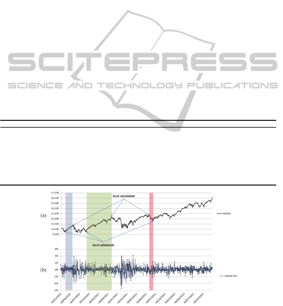
“Fig.1.b”, in which we have the daily percentage

changes of the DJIA30 Index, due to very small up

and down fluctuations of the stock market we have

extreme noise and it is very difficult to find meaning-

ful turning points (minima/maxima) that will signal a

trend reversal and a possible opportunity for buying

or selling stocks.

Our method, Moving Linear Regression Angle

analysis (MLRA), is based on the continuous execu-

tion of sliding linear regression analysis over time.

We perform continuous regression analysis of spe-

cific time interval-sliding window (width-data points)

and in each loop we calculate the angle of the regres-

sion line with the x-axis (the time axis of the time se-

ries) from the slope of the regression line. Assuming

that we have a time series of  data points we start at

the beginning of time 





0. Then for a specific

time interval, e.g. for stock prices this can be charac-

terized by 10 days (if the time series is ex-

pressed in days), we perform a linear regression anal-

ysis for data points up to 





9 (sliding window 0

to 9). Then we increase the starting point by one, i.e.,







1 and the ending point will become 





10

(sliding window 1 to 10). We continue this process

until we reach the end of the time series (sliding win-

dow 10 to 1, assuming the length of the time

series is ). In each loop we calculate the slope of the

regression line, and based on this the angle of the line

with respect to the x-axis in radius /2, /2.

With this process we construct a new time series of

 points and with starting point at 



and ending

point at 



of the original time series. In the new

time series, the value of the angles can show us how

the segments of the original time series behave re-

garding their monotony. If the angle of each part is

larger than the previous then the specific part of width

w has an uptrend while if it is smaller it has a down-

trend. When the values change from larger to smaller

we have a local maximum while when they change

from smaller to larger we have a local minimum

“Fig.1.a”.

Table 1: Identicative Results of Repeated Patterns in DJIA30 Transformation for MLRA10.

Index Pattern Start Period Occ. Length Positions

ZZZZZZZZZZZZZAAAAAAAAAAAAAAAAAAAAAAAAAAAAAAAAAAAA

155 783 2 49 155,938

ZZZZZZZZZZZZAAAAAAAAAAAAAAAAAAAAAAAAAAAAAAAAAAAA

219 720 2 48 219,939

AAAAAAAAAAAAAAAAAAAAAAAAAAAAAAAAAAAAZZZZZZZZZ

251 700 2 45 251,951

ZZZZZZAAAAAAAAAAAAAAAAAAAAAAAAAAAAAAAAA

225 524 2 39 225,749

ZZZZZZZZZZZAAAAAAAAAAAAAAAAAAA

435 505 2 30 435,940

AAAAAAAAAAAAAAAAAAAZZZZZZZZZAA

268 379 2 30 268,647

AAAAAAAAAAAAAAAAAAAAZA

59 820 2 22 59,879

ZZZZZZZZZZZZZZZZZZZZZZ

347 557 2 22 347,904

AAAAAAAAAAAAZZZZZZZZZZZZZZZZ

0 578 2 28 0,578

AAAAAAAAAAAAAAAAAAAA

267 231 4 20 267,498,729,960

Figure 1: Dow Jones Industrial Average 30 Prices and Daily Percentage Changes for 2010-2013.

ICEIS2015-17thInternationalConferenceonEnterpriseInformationSystems

348

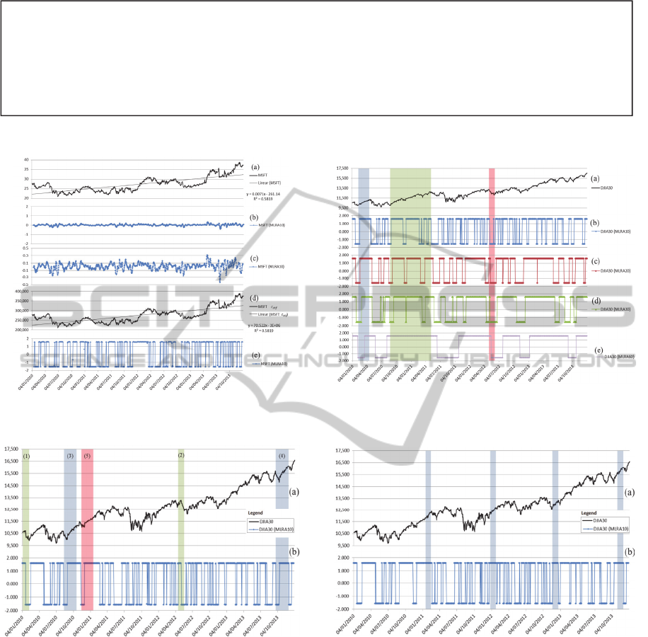
Figure 4: Discretized Time Series for DJIA30 for 2010-2013 using MLRA for 10 days interval.

Figure 2: Microsoft Stock Prices and MLRA Transfor-

mations for years 2010-2013.

Figure 3: Dow Jones Industrial Average 30 Prices an

MLRA Transformations for 2010-2013.

Figure 5: DJIA30 Transformed Time Series and Trend De-

tection Examples.

Figure 6: DJIA30 Transformed Time Series and Trend De-

tection Examples.

However, there is a significant obstacle when we deal

with time series having their values very small and

close to the slope of the regression line, and based on

this the angle of the line with respect to the x-axis. In

“Fig.2.a” we have the stock prices for Microsoft from

January 4th, 2010 till December 31st, 2013. The val-

ues vary between $20 and $40. As we can observe in

“Fig.2.b” the values in the new time series created by

applying the proposed MLRA change very smoothly.

In “Fig.2.c” we can see how the values fluctuate very

close to 0. So far the new time series behaves exactly

like the original time series and it is very difficult to

detect the local minima/maxima and the change in

trends. In order to make this process easier algorith-

mically, we will use a transformation on the original

time series. For the transformation, we will multiply

the original time series with a constant, which we will

name Sharpness Transformation Factor, denoted





, in order to move away the time series from the

. Doing this we will not lose any information

of the original time series, however, the regression

lines of each MLRA phase will become much steeper.

As we can see in “Fig.2.d”, we have the transformed

Microsoft stock prices and in “Fig.2.e” we have the

AAAAAAAAAAAAZZZZZZZZZZZZZZZZZZAAAAAAAAAAAAAAAAAAAAAAAAAAAAAAAAAAAAAAAAAAAAAAAAAZAZZZZZZZZZZZZZZZZZZZZZZZAZZZZZZAAAA

AAAAZZZZZZZZZZAAAAAAAAZZZAAAAAAAAAAAAAZZZZZZZZZZZZZZZAAAAAAAAAAAAAAAAAAAAAAAAAAAAAAAAAAAAAAAAAAAAAAAAAAAZZZZZZZZ

ZZZZAAAAAAAAAAAAAAAAAAAAAAAAAAAAAAAAAAAAAAAAAAAAAAAAAAAAAAAAZZZZZZZZZAAZZZZZZZZZAAAAAAAAAAAAAAZZZZZZZAAAAAAAAAA

AZZZZZZZZZZZZZZZZZZZZZZZZZZZZZZAAAAAAAAAAAAAAAAZZZZZAAAAAZZZZZZZZZZZZZZAAAZZZZZAAAAAAAZZZZZZAAAAAZZZZZZZZZZZAAAAAAAAAAA

AAAAAAAZAAZZAAAZZZZZZZZZZAAAAAAAAZZZZZZZAAAAAAAAAAAAAAAAAAAAAAAAAAZZAAAAAAAAAZAAAAAAAAAAAZZZZZAAAAAAAAZZZZZAAAAZ

ZZZZZZZAAAAAAAAAAAAAZZZZZZZZZZZZZZZZAAZZZZZZAAAAAAAAAAAZZZZAAAAAAZZZZZAAAAAZZAAAAAAAAAAAAAAAAAAAZZZZZZZZZAAAAAAAAAA

AAAAZZZZZZZAAAZZZZZZAAAZZZZZZZZAAZZZZZZZZZZAAAAAAAAAAAAAAAAAAAAAZZZZZZAAAAAAAAAAAAAAAAAAAAAAAAAAAAAAAAAZZZZZAAAAA

AAAAAAAAAAAAZAAAAAAAAAAAAAAAAZZZZZZAAAAAAAAAAAAAAAAAAAAAAAAZZZZZZZZZZZAAAZZZZZZZZAAAAAAAAAAAAAAAAAAAAZAAAAZZZZZ

ZZZZZZZZZZZZZZZZZAAAAAAAAAAAAZZZZZZZZZZZZZAAAAAAAAAAAAAAAAAAAAAAAAAAAAAAAAAAAAZZZZZZZZZZAAAAAAAAAAAAA

DiscretizationMethodfortheDetectionofLocalExtremaandTrendsinNon-discreteTimeSeries

349

MLRA transformation for 



 10,000. The choice

of the specific value for the 



is not critical since

we have used this for two reasons (a) we have exper-

imentally observed that when the values of a time se-

ries is above 100,000 then the regression lines of the

MLRA are very steep and the identification of the

slopes is more obvious and accurate; and (b) it is pre-

ferred to use multiples of 10 (or power of 10) as 



because this transforms the original value to a multi-

ple of 10 and the values remain recognizable. For ex-

ample, with Microsoft’s stock prices in “Fig.2.a” the

values are between 20 and 40 while in the trans-

formed time series with 



 10,000 the values are

between 200,000 and 400,000 as shown in “Fig.2.d”.

It is easy to translate a transformed value of 278,800

for January 4

, 2010 to 27.88 which is the actual

value of the original time series. Moreover, the anal-

ogy between values has not changed since for in-

stance between January 4

and January 5

, 2010 the

percentage change is 0.036% (from $27.88 to

$27.89), while in the transformed time series the

change is also 0.036% (from 278,800 to 278,900). We

can observe that the time series diagram is exactly the

same except that if we apply a linear regression anal-

ysis in both lines we have a slope and intercept of

10,000 times larger for the transformed time series.

However, the important outcome of the transfor-

mation can be observed in “Fig.2.c” and “Fig.2.e”. In

“Fig.2.c” we have the original MLRA time series

which fluctuates very smoothly around 0 while in

“Fig.2.e” we have the new time series constructed by

the MLRA on the transformed time series. The sec-

ond MLRA time series gives extreme values for the

angles which are mainly close to /2 and /2 with

very few exceptions. In this case, having the values

close to /2 means that we have a positive slope and,

therefore, an uptrend while being close to /2

means a negative slope and, therefore, a downtrend.

In order to verify that the time series characteris-

tics have not changed we can check how the actual

values are changing. This specific transformation of

type 



∗ does not alter the time series in

a way to produce false outcome. The only noticeable

change is the absolute Euclidean distance between the

points. For example, if we have the points (1,1) and

(2,2) they form a line with a slope of 45 degrees with

the x-axis (). If we multiply the y-coordinates

by 10 then we have two new points (1,10) and (2,20)

that form a new line with approximately 84 degrees

slope with the x-axis (10∗). The only change

is the Euclidean distance between the points which

now is

√

101

instead of

√

2. However, when analyz-

ing time series we care mostly about the relative

positions, i.e., how the analogies between the points

stand. In the specific example the change in the first

case is 100% (from 1 to 2) and the same is in the sec-

ond case (from 10 to 20).

Our method although gives direct information

about the trends of the segments of a time series it can

also provide more information. For example, when a

trend changes the specific point has to be either a lo-

cal minimum or a local maximum. Based on this we

can find the actual points in the time series and calcu-

late the time lag  between two changing points

(min-max or max-min) and find also the value change

 (difference of the two points on the y-axis). Based

on these two observations we can calculate the inten-

sity of the trend, i.e., how fast or slow it changes and

towards which direction. For example an upward

change of 100% in 10 days is more intense and im-

portant than the same change over 100 days (“Fig.1”).

Based on the above method, we can discretize the

new MLRA time series using a three letters alphabet,

e.g., A for values in 1, /2 , Z for values in

/2, 1 and O for values in 1,1. Type O val-

ues are very rare and we can eliminate them if we use

a different 



value which will create even steeper

linear regression lines. After we have created the new

MLRA time series we will apply ARPaD Algorithm

(Xylogiannopoulos et al., 2014), which is an im-

provement of COV Algorithm (Xylogiannopoulos et

al., 2012; 2014) and allows the detection of all re-

peated patterns in a time series. The ARPaD Algo-

rithm is the only algorithm that can detect all repeated

patterns in a very efficient time. This has been proven

experimentally with the analysis of 100 million deci-

mal digits for each one of the four most famous math-

ematical constants (π, e, φ,

√

) and for which ARPaD

managed to detect all repeated patterns (Xylogi-

annopoulos et al., 2014). After detecting the repeated

patterns we can use a periodicity detection algorithm

(Rasheed et al., 2010) in order to check for periodici-

ties in the previously detected repeated patterns.

4 EXPERIMENTS

For our experiments we used a PC with a double core

CPU at 2.6GHz and 4GB RAM. We have conducted

experiments on the Dow Jones Industrial Average 30

Index for the period from January 4th, 2010 until De-

cember 31st, 2013. We have performed 4 different

experiments using different time intervals and more

specifically we have used MLRA for 10, 20, 30 and

60 days. In “Fig.3.a” we can see the actual DJIA30

time series while in “Fig.3.b” through “Fig.3.d” we

ICEIS2015-17thInternationalConferenceonEnterpriseInformationSystems

350

have the different MLRA time series. From the dia-

grams we can make two observations. First, we can

see that indeed the MLRA detects the trends of the

original DJIA30 time series, e.g., in the three shaded

regions we have marked on the diagram. The first two

show an uptrend while the third a downtrend. We can

see that MLRA(10) shows exactly the trends and ad-

ditionally for the second time period (shaded region)

it detects also smaller downtrends (short-term analy-

sis) in the main uptrend. These fluctuations have been

eliminated in MLRA(60) because by taking a larger

time interval we actually eliminate the noise of the

small fluctuations of the index in the specific time pe-

riod (long-term analysis). The second thing we can

observe is that we have a lag between the actual turn-

ing point (local minimum or maximum) and therefore

the change of the trend and the change of the MLRA

values. Actually the larger the MLRA interval the

larger the lag. This is normal since MLRA is the lin-

ear regression of past values in time. The more data

points we use for the linear regression analysis in

MLRA the later the change will be observed. How-

ever, the lag is always the same for each analysis (de-

pending on the time interval). Therefore, when we

conduct a pattern and periodicity detection we have

just to move the turning point detected by the MLRA

specific data points back, according to the length of

the MLRA analysis.

In “Fig.4” we have the transformed time series

constructed by the MLRA(10) process (ten days in-

terval for the DJIA30). With A we have values close

to /2 while with Z we have values close to /2.

By conducting pattern detection with the ARPaD al-

gorithm (Xylogiannopoulos et al., 2014) and perio-

dicity detection with the PDA algorithm (Rasheed et

al., 2010) we have found many long patterns that in-

dicate potential periodicities for forecasting purposes.

In Table 1, we have some indicative results for pat-

terns with periodicity confidence 1 and length equal

to or larger than 20 days. We have included the posi-

tions at which the patterns occur and also calculated

the period of the occurrences. As an example, for the

pattern

“AAAAAAAAAAAAZZZZZZZZZZZZZZZZ” (in-

dex 9) we can see that it starts at position 0 and repeats

with a period of 578 days. It has to be mentioned that

financial time series are referring to working and not

calendar days and, therefore, periods are calculated

over working days too. Moreover, in the specific ex-

periments we have few data prior to January 4

, 2010

and therefore the position 0 of MLRA(10) indicates

the angle of the linear regression for the nine last days

of 2009 and January 4

, 2010 of DJIA30. If we check

the diagram we can see that DJIA starts at 2010 with

an uptrend of 12 days followed by a downtrend of 16

days. The specific pattern repeats again on April 19th,

2012 (shaded regions (1) and (2) “Fig.5”) and it is ex-

pected to occur again at the end of July 2014. For the

longest repeated pattern we have discovered (index 1)

it occurs for the first time on August 16th, 2010 with

a downtrend for 13 days followed by an uptrend of 36

days. The specific pattern occurs again on September

26th, 2013 (shaded regions (3) and (4) “Fig.5”) with

a period of 783 days and it is expected to occur again

at the beginning of November 2016. Almost a similar

pattern of 48 days (instead of 49) with a downtrend of

12 days (instead of 13) followed by an uptrend of 36

days (index 2) occurs first on November 15th, 2010

(shaded region (5) “Fig.5”) and then again on Sep-

tember 26th, 2013 (shaded region (4) “Fig.5”) with a

period of 720 days and it is expected to occur again at

the middle of July 2016. Another interesting trend is

20 days of uptrend occurring 4 times with a period of

231 days and first occurrence on January 25th, 2011,

second on December 22nd, 2011, third on November

26th, 2012 and the last on October 25th, 2013 (index

10, shaded regions “Fig.6”). For the specific last out-

come, we expect to have the same trend occurring at

the end of September 2014. As we can see, our

method can be used not just for forecasting purposes

of the next data point, but also to make forecasts

longer in the future time.

5 CONCLUSIONS

In this paper, we introduce a new discretization

method for the real values of a time series that allows

detecting local extrema and trends inside the time se-

ries. The proposed method is based on the transfor-

mation of the values of the original time series and

then the construction of a new time series from the

angle of the regression lines that are produced each

time we run a linear regression analysis in a sliding

window of short time intervals. The specific method

can be applied on all kind of real values time series,

e.g., meteorological data, traffic, internet, economic,

etc. We have conducted experiments for different

time intervals of 10, 20, 30 and 60 days on the prices

of Dow Jones Industrial Average 30 Index from the

beginning of 2010 until the end of 2013. After the dis-

cretization and formation of the new time series, we

conducted pattern and periodicity detection. The ex-

perimental results have proven the correctness and

consistency of the method in order to detect trends in

time series and through them to perform forecasting

based on historical data.

Furthermore, as we have discussed, this method

DiscretizationMethodfortheDetectionofLocalExtremaandTrendsinNon-discreteTimeSeries

351

can detect the local minima and maxima and through

them perform deeper analysis of the trends. More spe-

cifically, we can find the intensity of the trend (i.e.

how fast or slow it changes) and the overall perfor-

mance of the trend (i.e., the percentage change from

the minimum to the maximum data point or the rever-

sal). The specific process needs, besides the trend de-

tection, the actual minima and maxima values over

the time series and more calculations on the trends’

data values. Such process will be extensively ana-

lyzed in future work.

REFERENCES

Balkin, S.D., Ord, K., 2000. Automatic Neural Network

Modeling for Univariate Time Series. International

Journal of Forecasting, (1)6,4, pp. 509-515.

Bao, D., 2008. A Generalized Model for Financial Time Se-

ries Representation and Prediction. Applied Intelli-

gence, (29), pp. 1-11, doi: 10.1007/s10489-007-00631.

Bao, D.N., Vy, N.D.K., Anh, D.T., 2013. A hybrid method

for forecasting trend and seasonal time series. 2013

IEEE RIVF International Conference on Computing

and Communication Technologies, Research, Innova-

tion, and Vision for the Future (RIVF), pp.203-208.

Chen, Y.S., Cheng, C.H., Tsai, W.L., 2014. Modeling Fit-

ting-Function-Based Fuzzy Time Series Patterns for

Evolving Stock Index Forecasting. Applied Intelli-

gence, doi: 10.1007/s10489-014-0520-6.

De Gooijer, J.G., Hyndman, R., 2006. 25 Years of Time Se-

ries Forecasting. International Journal of Forecasting,

(22), pp. 443-473.

Edwards, R., Magee, J., Bassetti, W.H.C., 2007. Technical

Analysis of Stocks and Trends. CRC Press. 9

edition.

Esling, P., Agon, C., 2012. Time-Series Data Mining. ACM

Computing Surveys (CSUR), (45)1,12.

Gardner, E.S.Jr., McKenzie, E., 1985. Forecasting Trends

in Time Series. Management Science, (31)10, pp. 1237-

1246.

Guerrero, V.M., Galicia-Vasquez, A., 2010. Trend Estima-

tion of Financial Time Series, Applied Stochastic Mod-

els in Business and Industry, (26), pp. 205-223.

Kovalerchuck, B., Vityaev, E., 2000. Data Mining in Fi-

nance: Advances in Relational and Hybrid Methods.

Kluwer Academic Publishers, ISBN 0792378040.

Muhlbauer, A., Spichtinger, P., Lohmann, U., 2009. Appli-

cation and Comparison of Robust Linear Regression

Methods for Trend Estimation. Journal of Applied Me-

teorology and Climatology [1558-8424] Spichtinger,

Peter, (48)9, pp.1961-1970.

Muller, K.R., Smola, J.A., Scholkopf, B., 1997. Prediction

Time Series with Support Vector Machines[C]. In Pro-

ceedings of International Conference on Artificial Neu-

ral Networks, Lausanne, pp. 999-1004.

Pring, M., 2002. Technical Analysis Explained. McGraw-

Hill. New York, NY, 4

edition. ISBN 0071226699.

Qin, L.P., Bai, M., 2009. Predicting Trend in Futures Prices

Time Series Using a New Association Rules Algorithm.

International Conference on Management Science

& Engineering 2009, pp. 1511-1517.

Rasheed, F., Alshalfa M., Alhajj, R., 2010. Efficient Perio-

dicity Mining in Time Series Databases Using Suffix

Trees. IEEE TKDE, (22)20, pp. 1-16.

Selvaratnam, S., Kirley, M., 2006. Predicting Stock Market

Time Series Using Evolutionary Artificial Neural Net-

works with Hurst Exponent Input Windows[C]. Ad-

vances in Artificial Intelligence, pp.617-626.

Xi-Tao, W., 2006. Study on the Application of ARIMA

Model in Time-Bargain Forecast[J]. E-Commerce and

Logistics, 22(15)139-140H.

White, H., Granger, C.W.J., 2011. Consideration of Trends

in Time Series, Journal of Time Series Econometrics,

(3)1,2.

Xylogiannopoulos, K., Karampelas, P., Alhajj, R., 2012.

Periodicity Data Mining in Time Series Using Suffix

Arrays, in Proc. IEEE Intelligent Systems IS’12.

Xylogiannopoulos, K., Karampelas, P., Alhajj, R., 2014.

Exhaustive Patterns Detection In Time Series Using

Suffix Arrays. , manuscript in submission.

Xylogiannopoulos, K., Karampelas, P., Alhajj, R., 2014.

Analyzing Very Large Time Series Using Suffix Ar-

rays, Applied Intelligence, (41)3, pp. 941-955.

Xylogiannopoulos, K., Karampelas, P., Alhajj, R., 2014.

Experimental Analysis on the Normality of pi, e, phi

and square root of 2 Using Advanced Data Mining

Techniques. Experimental Mathematics, (23)2.

Yang, Y., Webb, G., Wu, X., 2005. Data Mining and

Knowledge Discovery Handbook, Chapter 6. Springer.

ICEIS2015-17thInternationalConferenceonEnterpriseInformationSystems

352