
Automatic Representation and Classifier Optimization for Image-based
Object Recognition
Fabian B¨urger and Josef Pauli
Lehrstuhl f¨ur Intelligente Systeme, Universit¨at Duisburg-Essen, Bismarckstraße 90, 47057 Duisburg, Germany
Keywords:
Manifold Learning, Model Selection, Evolutionary Optimization, Object Recognition.
Abstract:
The development of image-based object recognition systems with the desired performance is – still – a chal-
lenging task even for experts. The properties of the object feature representation have a great impact on the
performance of any machine learning algorithm. Manifold learning algorithms like e.g. PCA, Isomap or
Autoencoders have the potential to automatically learn lower dimensional and more useful features. How-
ever, the interplay of features, classifiers and hyperparameters is complex and needs to be carefully tuned
for each learning task which is very time-consuming, if it is done manually. This paper uses a holistic opti-
mization framework with feature selection, multiple manifold learning algorithms, multiple classifier concepts
and hyperparameter optimization to automatically generate pipelines for image-based object classification. An
evolutionary algorithm is used to efficiently find suitable pipeline configurations for each learning task. Exper-
iments show the effectiveness of the proposed representation and classifier tuning on several high-dimensional
object recognition datasets. The proposed system outperforms other state-of-the-art optimization frameworks.
1 INTRODUCTION
The object recognition problem widely occurs in
many relevant real-world applications like optical
character recognition (OCR), robotic vision or driver
assistance systems. The human visual system has ex-
traordinary pattern recognition capabilities and can
perform many of the aforementioned tasks effort-
lessly. There is currently no general purpose com-
putational model for object recognition with similar
capabilities. Generally, object recognition is subdi-
vided into object segmentation, feature extraction and
classification. This paper aims at an automatic opti-
mization of the last two aspects in a holistic manner.
The input data is low-level and noisy pixel data
which is usually not invariant to e.g. scale, rotation
or illumination changes. The properties of the fea-
ture representation have a tremendous effect on the
classifier performance. Some popular standard fea-
tures exist, e.g. SIFT (Lowe, 2004) or Local Binary
Patterns (Ojala et al., 2002), which provide a reason-
able degree of invariance. However, in many cases
task-specific features have to be developed manually
to fulfill the performance requirements.
The field of representation learning is focused
on the analysis and automatic construction of good
features for machine learning (Bengio et al., 2013).
There are multiple approaches to learn new fea-
tures; deep neural networks (Ngiam et al., 2011)
have shown a great success in fields of object and
speech recognition. Manifold learning is a promis-
ing approach to generate lower-dimensional features
that potentially circumvent the curse of dimensional-
ity. There are numerous different algorithms based on
e.g. statistical analyses, neural networks or neighbor-
hood graphs, and their performance heavily depends
on the learning task. The interplay of selected fea-
tures, manifold learning algorithms, classifiers and
hyperparameters
1
is very complex and needs to be
carefully adapted for each learning task.
In order to tackle the burden of manual optimiza-
tion this paper uses a holistic optimization pipeline
with all the aforementioned components recently pro-
posed in (B¨urger and Pauli, 2015). The framework
contains portfolios for manifold learning algorithms
and multiple classifier concepts. The extremely large
search space of this optimization problem is handled
with evolutionary algorithms so that optimized pro-
cessing pipelines can be obtained within a few hours
on a normal workstation computer. The huge degree
of adaptability bears the risk of overfitting to the train-
1
Hyperparameters influence a learning algorithm itself,
like the regularization parameter C in a support vector ma-
chine (SVM).
542
Bürger F. and Pauli J..
Automatic Representation and Classifier Optimization for Image-based Object Recognition.
DOI: 10.5220/0005359005420550
In Proceedings of the 10th International Conference on Computer Vision Theory and Applications (VISAPP-2015), pages 542-550
ISBN: 978-989-758-090-1
Copyright
c
2015 SCITEPRESS (Science and Technology Publications, Lda.)

ing set which is tackled in two ways: The general-
ization of the manifold learning algorithm is incor-
porated in the cross-validation process. Additionally,
the variation of the best solutions of the evolutionary
algorithm is exploited to build a multi-pipeline classi-
fier.
The proposed framework already showed promis-
ing results on rather low-dimensional (4–60 dimen-
sions) classification datasets from the UCI database
(Bache and Lichman, 2013). This paper presents
improvements on the framework and experiments on
high-dimensional (256–1370 dimensions) real-world,
multiclass object recognition tasks. The performance
of automatically learned features out of low-level fea-
tures is compared with standard high-level features.
Also, the impact of the portfolio of manifold learning
algorithms is evaluated. Finally, comparisons to the
state-of-the-art optimization framework Auto-WEKA
(Thornton et al., 2013) are made.
2 RELATED WORK
The field of object recognition is too large to give an
extensive overview of the topic. This section focuses
on feature construction methods and automatic opti-
mization of machine learning systems.
2.1 Feature Construction and Manifold
Learning
Manifold learning and dimension reduction feature
transforms are one aspect of representation learning.
The basic idea is to feature distributions typically do
not fill all dimensions equally, but contain areas of
lower-dimensional structures that are embedded in the
high dimensional space. Manifold learning makes
use of these geometrical structures and correlations to
learn a model to transform high-dimensional feature
vectors into the intrinsic lower dimensional space.
There are numerous different linear and non-linear
manifold learning algorithms; a list of common meth-
ods and references can be found in the appendix. The
work of (Van der Maaten et al., 2009) and (Ma and
Fu, 2011) provide an overview of these methods.
These algorithms base on completely different ap-
proaches – e.g. neural networks, statistical analyses,
kernel methods, neighborhoodgraphs –, but they fit to
a generalized feature transform interface f
FeatTrans
: A
training set T is given with 1 ≤ i ≤ m feature vectors
x
i
∈ R
D
and class labels y
i
∈ {ω
1
,ω
2
,...,ω
c
}. Note
that most manifold learning algorithms are unsuper-
vised and thus ignore the labels. A manifold learning
algorithm to reduce the dimensionality from D to d
can expressed with a learning function
M = f
learn
(T,d) (1)
that derives the model variables M. The transform
function
˜
x = f
trans
(x,M) ∈ R
d
(2)
embeds a vector x ∈ R
D
into the new subspace using
the model M.
In real-world applications, there are several prob-
lems with manifold learning algorithms. First, the
feature transform function must be capable of em-
bedding previously unseen feature vectors to allow
an out-of-sample extension. Linear methods use a
transformation matrix and can extend any vector,
but many non-linear methods lack a direct extension
method. The Nystr¨om theorem (Bengio et al., 2003)
can be used to estimate this extension for methods that
rely on spectral decompositions like LLE, Isomap or
Laplacian Eigenmaps. Furthermore, many methods
work well for artificial datasets, but fail to produce
useful features on noisy real-world datasets as exper-
iments in (Van der Maaten et al., 2009) show.
2.2 Automatic Machine Learning
Optimization
Automatic optimization frameworks aid developersto
select suitable features, classifier concepts and hyper-
parameters which is often referred to as model se-
lection problem. The more components contain de-
grees of freedom, the more complex the optimiza-
tion gets and only few publications deal with holis-
tic approaches. Usually, search-based meta heuris-
tics are used to find solutions within a reasonable
time. In (Huang and Wang, 2006) and (Huang and
Chang, 2007) “classical” feature selection is com-
bined with hyperparameter optimization of a single
classifier using evolutionary algorithms (see section
4.2). The Auto-WEKA framework (Thornton et al.,
2013) aims to solve the combined feature selection,
classifier selection and hyperparameter optimization
problem using a Bayesian approach. It provides the
most comprehensive amount of optimized compo-
nents as it relies on the numerous algorithms con-
tained in the WEKA machine learning framework
(Hall et al., 2009). Therefore, Auto-WEKA will be
compared in the experiment section in section 5.
However,Auto-WEKA does not contain the selec-
tion of manifold learning or feature transform meth-
ods. In (B¨urger and Pauli, 2015), we introduced a
holistic optimization framework for feature selection,
multiple feature transforms, multiple classifiers and
hyperparameters that uses evolutionary algorithms.
This framework is briefly described in the following.
AutomaticRepresentationandClassifierOptimizationforImage-basedObjectRecognition
543
Feature
Transform
Element
Classifier
Element
Class
Label
Feature
Selection
Element
Input
Instance
Feature
Scaling
Element
Figure 1: Classification pipeline structure (B¨urger and Pauli, 2015).
3 HOLISTIC CLASSIFICATION
PIPELINE
The framework proposed in (B¨urger and Pauli, 2015)
provides a connection between classifier with hyper-
parameter selection, feature selection and automatic
feature construction methods while the last two as-
pects are considered as representation optimization.
The central processing algorithm is based on a classi-
fication pipeline framework which is described in the
following subsections.
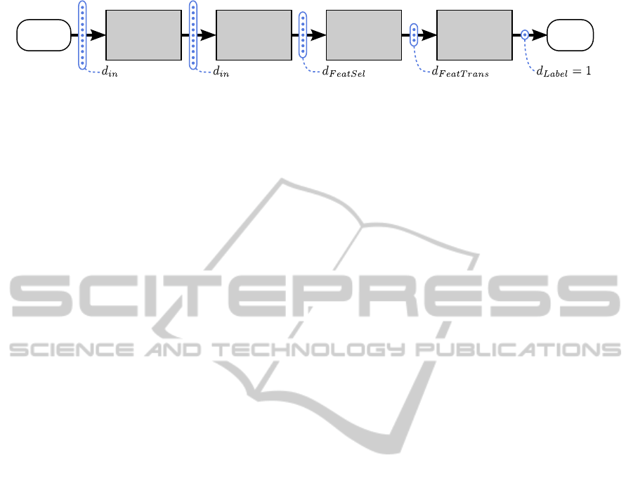
3.1 Pipeline Structure
The classification pipeline structure contains four
pipeline elements that are depicted in figure 1. It
has basically two modes – first, the training mode in
which the training dataset T is used to adapt and train
all pipeline elements. In the classification mode new
feature vectors are classified with the trained pipeline.
The general processing concept of the pipeline is con-
secutive dimension reduction after each pipeline ele-
ment:
d
in
≥ d
FeatSel
≥ d
FeatTrans
≥ d
Label
= 1. (3)
3.1.1 Feature Scaling Element
The first pipeline element performs a rather simple
feature scaling to a value range of [0,1] based on the
minimum and maximum values in T. This prepro-
cessing step usually leads to a performance improve-
ment for all machine learning algorithms that rely on
distance metrics.
3.1.2 Feature Selection Element
The feature selection element is the first dimension
reduction in the pipeline and selects a subset of single
features S
FeatSet
∈ P ({1,2,...,d
in
}) \
/
0. The idea is
that this element removes any irrelevant features that
could possibly disturb any following algorithm. The
dimensionality of the remaining feature space is de-
noted as d
FeatSel
.
3.1.3 Feature Transform Element
The feature transform element is used to apply a
manifold learning algorithm f
FeatTrans
and finally
transform the data into a new feature space with di-
mensionality d
FeatTrans
. During training, one algo-
rithm is chosen out of a portfolio S
FeatTrans
(see ap-
pendix) and trained with the selected feature subset
S
FeatSet
of T. The portfolio S
FeatTrans
also contains the
identity function (or simply no transform) because all
other transformations might fail to produce more use-
ful features than the original ones.
3.1.4 Classifier Element
The last pipeline element selects a classifier f
Classifier
out of a portfolio S
Classifiers
of concepts listed in ta-
ble 1. The no-free-lunch theorem states that no single
classifier concept performs best for all learning tasks
and the potential of a good feature transform might
be lost if a suboptimal classifier concept is chosen. In
training mode, the transformed data from the previous
element is used to train the classifier. Note that each
classifier has its own set of independent hyperparam-
eters S
Params
( f
Classifier
) that can be of arbitrary type
(also see table 1).
3.2 Pipeline Configuration
The proposed pipeline has numerous degrees of free-
dom to adapt to each learning task. The most impor-
tant parameters are summarized in the pipeline con-
figuration
θ = (S
FeatSet
, f
FeatTrans
,d
FeatTrans
,
f
Classifier
,S
Params
( f
Classifier
)), (4)
namely the selected feature subset S
FeatSet
, the mani-
fold learning algorithm f
FeatTrans
and its target di-
mensionality d
FeatTrans
as well as the classifier con-
cept f
Classifier
and its corresponding hyperparameters
S
Params
( f
Classifier
).
VISAPP2015-InternationalConferenceonComputerVisionTheoryandApplications
544
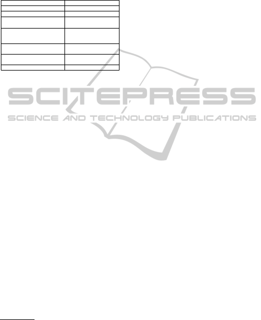
Table 1: Popular classifier concepts and corresponding hy-
perparameters and ranges. References to these classifier
concepts can be found e.g. in (Bishop and Nasrabadi, 2006)
and (Huang et al., 2006).
Classifiers parameter ranges
Naive Bayes -
C-SVM linear kernel C : [10
−2
,10
4
]
C-SVM Gaussian kernel C : [10
−2
,10
4
],
γ : [10
−5
,10
2
]
k nearest neighbors (kNN) k : [1,20], metric:
{Euclidean, Mahalan.,
Cityblock, Chebychev}
Multilayer Perceptron (MLP) hidden layers: [0,3],
neurons per layer: [1,10]
Extreme Learning Machine
(ELM)
neurons per layer: [1,200]
Random Forest number trees: [1,100]
4 OPTIMIZATION ALGORITHM
The search space of all possible configurationsis huge
as it contains feature selection with exponential com-
plexity O(2
d
in
) and the combinations of all manifold
learning algorithms, classifiers and hyperparameters.
The optimization approaches presented in (B¨urger
and Pauli, 2015) and improvements are described in
the following.
4.1 Target Function
In order to prevent overfitting, a suitable optimization
target metric based on a wrapper
2
approach combined
with k-fold cross-validation (Jain et al., 2000) is em-
ployed. The training dataset into divided into k sub-
sets and k validation rounds are made. In each round
k − 1 subsets are used for training and one is left out
for validation.
The manifold learning algorithm has a great im-
pact on the performance of the whole pipeline as
a non-linear feature transform may inherit parts of
the classifier’s “intelligence” as a linear classifier
model might be sufficient. However, if the mani-
fold learning is only used as a preprocessing step and
is not involved into the cross-validation, the gener-
alization of the out-of-sample function is never mea-
sured. Therefore, the manifold learning algorithm has
to be considered in each validation round. The train-
ing set is separated into k = 5 training and validation
tuples {(T
train,l
,T
valid,l
)}. In each cross-validation
round 1 ≤ l ≤ k, the selected manifold learning al-
gorithm is trained with T
train,l
and the out-of-sample
extension transforms the test and validation dataset
– separately – into the new feature space denoted as
2
In a wrapper approach a classifier is trained and its ac-
tual predictions are evaluated.
(
˜
T
train,l
,
˜
T
valid,l
). The selected classifier is trained with
the transformed training dataset
˜
T
train,l
and the accu-
racy is measured with the predictions on the trans-
formed validation dataset
˜
T
valid,l
. The average accu-
racy of all cross-validation rounds is used as target
metric.
4.2 Optimization with Evolutionary
Strategies
Evolutionary algorithms (EA) are especially suitable
to solve complex optimization problems with high di-
mensional search spaces. The basic idea of EA is the
imitation of the biological evolution of species that
adapt to their environment over time while Evolution-
ary Strategies (ES) are one variant of EA that are es-
pecially capable to optimize sets of heterogeneouspa-
rameters (Beyer and Schwefel, 2002). The objective
function F(y) needs to be optimized with respect to
the object parameter set y. These parameter sets can
be any combination of different data types:
• numeric data types R
N
and Z
N
with length N and
corresponding minimum and maximum values,
• bit string data types B
N
with length N,
• categorical data types S = {s
1
,s
2
,...,s
N
S
} with N
S
items without any order.
ES uses populations of individuals containing param-
eter sets y. The optimization starts with random in-
dividuals which are evolved over time with the help
of the evolutionary operators selection, recombina-
tion and mutation. The fitness function f(y) evalu-
ates each individual and only the fittest survive and
generate offspring.
Figure 2 depicts a strategy to code the pipeline
configuration θ completely as parameter set y. The
feature subset S
FeatSet
is coded as bit string B
d
in
. The
manifold learning algorithm f
FeatTrans
and the classi-
fier concept f
Classifier
are both coded as categorical
type S. The target dimensionality d
FeatTrans
for the
manifold learner cannot be coded directly as it de-
pends on the number of selected features in S
FeatSet
.
Instead, a dimension fraction factor α ∈ [0,1] is used
for the coding and the target dimensionality is ob-
tained with
d
FeatTrans
= ⌊ α · d
FeatSel
⌋ , d
FeatTrans
≥ 1. (5)
The initial random values for α are sampled from a
smaller range of [0,0.1] which is a prior for lower di-
mensional feature spaces.
The structure of the classifier hyperparameter op-
timization problem S
Params
( f
Classifier
) is hierarchical
as the selection of a classifier concept f
Classifier
se-
lects the classifier specific set of hyperparameters(see
table 1).
AutomaticRepresentationandClassifierOptimizationforImage-basedObjectRecognition
545
Feature transform Dim. fraction
Feature subset
Classifier hyperparameters
Classifier
Figure 2: Exemplary coding schema of a pipeline configuration θ (B¨urger and Pauli, 2015).
In order to optimize all hyperparameters in a sin-
gle evolutionary way, the hierarchical problem is lin-
earized in the following way: All hyperparameters
of all classifiers are simply appended to the object
parameter set and evolved together. Exponentially
ranged hyperparameters (C and γ values for the SVM)
are optimized using the exponents log
10
(x). For the
evaluation of the fitness (see section 4.1), the pipeline
configuration uses those hyperparameters that belong
to the selected classifier f
Classifier
and simply neglects
the rest.
The parametrization of the ES optimization is
summarized in the (µ/ρ + λ) notation. The initial
population contains 500 random individuals and in
each generation λ = 200 individuals from ρ = 2 par-
ents are generated while the best µ = 50 individuals
survive. The mutation operator contains several prob-
ability parameters:
• the probability of bit flips for the feature selection
is p
bit flip
= 0.3,
• the probability of choosing a random item for all
parameters of the categorial type S is p
cat
= 0.3,
• for all numerical values, namely the α factor and
the classifiers’ hyperparameters, the mutation is
performed using an additive normally distributed
noise N (0,σ
2
). The standard deviation is adap-
tive to the value range of the corresponding hy-
perparameter with σ = 0.2 · (v
max
− v
min
).
The ES terminates if the improvement of the fit-
ness of the best individuals is less than ε = 10
−4
after
three consecutive generations.
4.3 Multi-pipeline Classifier
The result of an ES optimization is a set of config-
urations with corresponding fitness values {(θ
j
, f
j
)}.
This set can be sorted by the fitness values to obtain a
top list of configurations, such that θ
1
is the best so-
lution. Of course, this top configuration can be used
to set up a classification pipeline, but a single pipeline
can be problematic in the sense of overfitting. A sim-
ple solution is the fusion of multiple pipelines to a
multi classifier which generally leads to a better gen-
eralization when the diversity among the classifiers is
large enough (Ranawana and Palade, 2006). A multi-
pipeline classifier can easily be built with setting up
the top-n pipelines with the corresponding configura-
tions θ
j
with 1 ≤ j ≤ n. New instances are classified
by all pipelines and a majority voting is performed to
obtain the final label.
5 EXPERIMENTS
The proposed framework is tested on two real-world
image-based object recognition tasks with different
scenarios. The datasets contain low-level pixel fea-
tures and relatively few training instances compared
to the number of dimensions. This leads to the curse
of dimensionality which is a typical issue for image-
based classification tasks.
The focus of the experiments is the question what
role manifold learning plays and how different types
of features influence the performance. Three variants
of the proposed framework are evaluated:
• Manifold Learning Deactivated (ML: none): The
set S
FeatTrans
just contains the identity function.
• Only PCA (ML: PCA): The set S
FeatTrans
contains
the “popular” linear PCA and the identity.
• All Manifold Learning Methods (ML: All): The
set S
FeatTrans
contains all linear and non-linear
manifold learning algorithms listed in the ap-
pendix.
All datasets are separated randomly into 70% training
and 30% test data. The framework is implemented in
Matlab using the parallel computing toolbox. A base-
line SVM classifier with Gaussian kernel is used for
comparison as well as the Auto-WEKA framework
with 24 hours time budget.
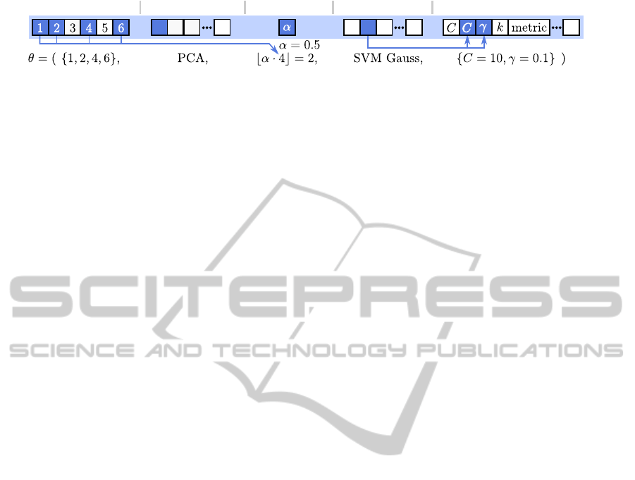
5.1 Classification of Coins
For this task, 5 different classes of Euro coins (1, 2,
5, 10 and 20 cent coins) need to be distinguished by
using RGB-color images. For each class, 16 differ-
ent coins are photographed from four different angles
leading to a total amount of 320 images. The coins are
segmented by simple thresholding (see figure 3) and
used to generate three datasets with different feature
sets:
VISAPP2015-InternationalConferenceonComputerVisionTheoryandApplications
546
Figure 3: Examples of the coins dataset.
Table 2: Training cross-validation accuracy values for the
coins datasets.
Low High Low+high
ML: none 69.78 85.78 83.56
ML: PCA
71.56 85.78 82.22
ML: All
68.44 93.78 92.00
Baseline 58.67 70.22 70.22
• Low-level Features. Normalized pixel values
(zero mean and standard deviation of 1) of 30×30
pixel images; total dimensionality: 900.
• High-levelFeatures. Area in pixels, statistical fea-
tures of gray and hue values in the HSV
3
space
(mean, standard deviation, skewness and kurto-
sis), histograms with 50 bins of gray and hue val-
ues, Local Binary Patterns in four variants: basic
(256 dimensions), uniform (59 dimensions), rota-
tion invariant (36 dimensions), rotation invariant
and uniform (10 dimensions); total dimensional-
ity: 470.
• Low+high-level Features. Low- and high-level
features together; total dimensionality: 1370.
5.1.1 Train and Test Performance
Table 2 lists the best cross-validation accuracy values
during training for all three frameworkvariants (rows)
and the three feature sets (columns). When all mani-
fold learning algorithms are used (variant ML: All) a
significant accuracy gain is achieved for the high- and
low+high-level features. Only for the low-level fea-
tures, the ML: PCA variant achieves the best result,
likely due to local minima during the optimization of
the full manifold learning algorithm portfolio. The
baseline SVM classifier is clearly outperformed in all
cases.
The optimization times on an Intel Xeon worksta-
tion with 6× 2.5 Ghz are listed in table 3. Due to the
larger search space and the high computation times of
some of the manifold learning algorithms (caused by
3
The Hue Saturation Value (HSV) color space is used to
analyze the color independently from brightness.
Table 3: Optimization times in minutes for the coins
datasets.
Low High Low+high
ML: none 19.2 29.7 46.9
ML: PCA
30.1 33.6 47.8
ML: All
314.7 224.4 911.7
Table 4: Generalization accuracy values on the test dataset
for the coins datasets (single top-1 configuration).
Low High Low+high
ML: none 78.95 83.16 83.16
ML: PCA
78.95 82.11 80.00
ML: All
75.79 84.21 92.63
Baseline 66.32 68.42 77.89
Auto-WEKA
72.63 89.47 92.63
the Matlab implementations), the total optimization
times are much larger for the ML: All variant.
Table 4 shows the generalization accuracy values
on the test dataset when the overall best configura-
tion is used. The proposed framework achievesa large
performance boost on the low-level feature set com-
pared to the training accuracy. The performance on
the high-level feature set is significantly lower. When
the low+high-level features are used, the accuracy on
the test dataset is in the same range than during train-
ing. Clearly, overfitting effects are responsible for
the partly relatively low generalization performance
of the proposed framework. The Auto-WEKA frame-
work performs best or equal on two of the three fea-
ture sets while the baseline SVM classifier shows a
poor performance on all feature sets.
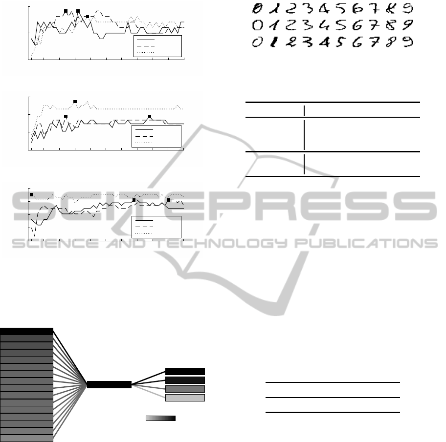
5.1.2 Multi-pipeline Classifier
The generalization performance values of the multi-
pipeline classifiers can be found in figure 4. A general
trend is visible: The performance is increasing when
more pipelines are used. Usually, a strong boost is
already achieved for less than 10 pipelines.
The distribution of the top configurations can con-
tain useful information about the classification prob-
lem. Figure 5 shows the top-50 configurations for the
ML: All framework variant on the low+high-levelfea-
ture set as a graph. The frequencies of the compo-
nents in the top solutions are denoted with different
shadings. In this case, only one manifold learning al-
gorithm is under the best solutions, namely the Large-
Margin Nearest Neighbor (LMNN) method. It is in-
teresting that the problem becomes linear as a linear
SVM showed the best performance. Furthermore, the
importance of the different features is easily visible
– in this case the area is the most important feature
AutomaticRepresentationandClassifierOptimizationforImage-basedObjectRecognition
547
number pipelines
1 5 10 15 20 25 30 35 40 45 50
accuracy
75
80
85
84.2184.21
83.16
ML: none
ML: PCA
ML: All
(a) Low-level features
number pipelines
1 5 10 15 20 25 30 35 40 45 50
accuracy
80
85
90
95
89.4789.47
93.68
ML: none
ML: PCA
ML: All
(b) High-level features
number pipelines
1 5 10 15 20 25 30 35 40 45 50
accuracy
75
80
85
90
95
90.53
90.53
92.63
ML: none
ML: PCA
ML: All
(c) Low+high-level features
Figure 4: Generalization accuracy values on the test dataset
of the multi-pipeline classifiers for the coins datasets de-
pending on the number of pipelines.
Area*
GrayValueStd*
colorHueStd*
GrayValueSkewness*
GrayValueMean*
LBP_RI_n8_r1*
LBP_Basic_n8_r1*
Pixels*
LBP_Uniform_n8_r1*
histogramColorHue*
histogramGray*
LBP_RIU_n8_r1*
colorHueMean
colorHueSkewness*
GrayValueKurtosis
colorHueKurtosis
LMNN*
SVM Gauss
SVM linear*
Random Forest
SVM Poly
Features Feature Transforms Classifiers
Frequency
Figure 5: Visualization of the top-50 configurations for the
coins dataset with low+high level features using the ML: All
variant. The overall best solution contains the items marked
with an asterisk.
which is not surprising as the coins have a different
size in reality. Also the contrast (gray value standard
deviation feature) is important.
5.2 Handwritten Digits
For the second experiment the semeion-digits dataset
(Buscema, 1998) from the public UCI database
(Bache and Lichman, 2013) is used. The dataset
contains 1593 samples of handwritten digits (0–9) in
Figure 6: Examples of the semeion-digits dataset.
Table 5: Accuracy on training and test dataset for the
semeion-digits dataset.
training dataset test dataset
ML: none 95.16 92.66
ML: PCA
95.16 93.50
ML: All
93.28 92.87
Baseline 93.46 92.03
Auto-WEKA
- 94.13
form of binary images with a size of 16× 16 pixels
(see figure 6). This leads to a 10-class problem with
a feature dimensionality of 256. In this dataset, only
the low-level pixel features are used.
5.2.1 Train and Test Performance
The training and test results are listed in table 5. It is
remarkable that the baseline SVM classifier already
performs very well on this dataset – the performance
gain of the proposed framework and Auto-WEKA is
marginal. The optimization times can be found in ta-
ble 6 and are higher because there are more training
samples compared to the coins datasets.
Table 6: Optimization times in minutes for the semeion-
digits dataset.
ML: none ML: PCA ML: All
28.8 99.0 1167.1
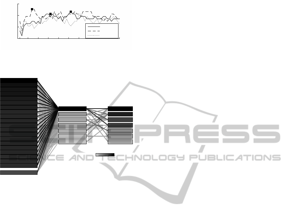
5.2.2 Multi-pipeline Classifier
The generalization performance of the multi-pipeline
classifiers (see figure 7) is slightly increasing with the
number of pipelines, and the best achievable perfor-
mance is better or equal to Auto-WEKA. However,
the performance gain is marginal for this dataset.
Figure 8 shows the distribution of the best config-
urations for the ML: All variant. The variety of well
performing manifold learning algorithms and classi-
fiers is large for this dataset.
6 CONCLUSIONS
This work presented improvements and extended
VISAPP2015-InternationalConferenceonComputerVisionTheoryandApplications
548
number pipelines
1 5 10 15 20 25 30 35 40 45 50
accuracy
92
93
94
95
94.34
94.55
94.13
ML: none
ML: PCA
ML: All
Figure 7: Generalization performance of the multi-pipeline
classifiers on the semeion-digits dataset.
F27*
F3
F187
F251
F16*
F123*
F208*
F40*
F58
F106*
F131
F141*
F155*
F160
F182*
F183*
F228
F9*
F35
F37
Rest (236 features)*
no transform*
LDA
NPE
NCA
PCA
Factor Analysis
LLE
SVM linear
kNN
SVM Gauss
Random Forest
ELM
SVM Poly*
Naive Bayes
Features Feature Transforms Classifiers
Frequency
Figure 8: Visualization of the top-50 configurations for the
semeion-digits dataset using the ML: All variant. The fea-
tures have linear numeric labels in this dataset.
evaluations of a holistic optimization framework for
feature selection, manifold learning, classifier and hy-
perparameter selection. The evaluations were per-
formed on image-based classification problems with
evident curse of dimensionality and different types of
feature sets. The results show that the proposed op-
timization methods find a reasonable pipeline config-
uration within a few hours. The benefit of the mani-
fold learning algorithms depends on the task and the
chosen features, but can be potentially large (see the
LMNN transform on the coins dataset). The type fea-
tures (low- vs. high-level) does not play a big role to
predict the success of manifold learning.
Overfitting effects are still noticeable even though
cross-validation is used. However, detailed stud-
ies of the multi-pipeline classifier showed a reason-
able boost in generalization performance, so that the
state-of-the-art optimization framework Auto-WEKA
is beaten for all datasets. However, the relatively
long optimization times are not always justifiable, if a
baseline SVM already performs very well.
Future work will focus on the improvement of
the optimization process in terms of speed and gen-
eralization. One approach can be the use of a fast
estimation algorithm at the beginning to generate a
better initial population. Furthermore, early rejec-
tion of inferior individuals during cross-validation is
a promising approach. A remedy against overfitting is
an increased diversity of configurations which can be
achieve with e.g. the extension of the evolutionary se-
lection operator with a maximum age of individuals.
Furthermore, alternativetarget metrics can be applied,
e.g. bootstrapping (Jain et al., 2000).
ACKNOWLEDGEMENTS
This work was funded by the European Com-
mission within the Ziel2.NRW programme
“NanoMikro+Werkstoffe.NRW”.
REFERENCES
Bache, K. and Lichman, M. (2013). UCI machine learning
repository. http://archive.ics.uci.edu/ml/.
Belkin, M. and Niyogi, P. (2001). Laplacian eigenmaps and
spectral techniques for embedding and clustering. In
Advances in Neural Information Processing Systems
(NIPS), volume 14, pages 585–591.
Bengio, Y., Courville, A., and Vincent, P. (2013). Represen-
tation learning: A review and new perspectives. Pat-
tern Analysis and Machine Intelligence, IEEE Trans-
actions on, 35(8):1798–1828.
Bengio, Y., Paiement, J.-f., Vincent, P., Delalleau, O., Roux,
N. L., and Ouimet, M. (2003). Out-of-sample exten-
sions for lle, isomap, mds, eigenmaps, and spectral
clustering. In Advances in Neural Information Pro-
cessing Systems, page None.
Beyer, H.-G. and Schwefel, H.-P. (2002). Evolution strate-
gies - a comprehensive introduction. Natural Comput-
ing, 1(1):3–52.
Bishop, C. M. and Nasrabadi, N. M. (2006). Pattern recog-
nition and machine learning, volume 1. Springer New
York.
Brand, M. (2002). Charting a manifold. In Advances in neu-
ral information processing systems, pages 961–968.
MIT Press.
B¨urger, F. and Pauli, J. (2015). Representation optimiza-
tion with feature selection and manifold learning in
a holistic classification framework. In International
Conference on Pattern Recognition Applications and
Methods (ICPRAM 2015, accepted), Lisbon, Portugal.
INSTICC, SCITEPRESS.
Buscema, M. (1998). Metanet*: The theory of independent
judges. Substance use & misuse, 33(2):439–461.
Donoho, D. L. and Grimes, C. (2003). Hessian eigen-
maps: Locally linear embedding techniques for high-
dimensional data. Proceedings of the National
Academy of Sciences, 100(10):5591–5596.
Fisher, R. A. (1936). The use of multiple measurements in
taxonomic problems. Annals of Eugenics, 7(2):179–
188.
AutomaticRepresentationandClassifierOptimizationforImage-basedObjectRecognition
549

Goldberger, J., Roweis, S., Hinton, G., and Salakhutdinov,
R. (2004). Neighbourhood components analysis. In
Advances in Neural Information Processing Systems
17.
Hall, M., Frank, E., Holmes, G., Pfahringer, B., Reutemann,
P., and Witten, I. H. (2009). The weka data min-
ing software: an update. ACM SIGKDD explorations
newsletter, 11(1):10–18.
He, X., Cai, D., Yan, S., and Zhang, H.-J. (2005). Neigh-
borhood preserving embedding. In Computer Vision
(ICCV), 10th IEEE International Conference on, vol-
ume 2, pages 1208–1213.
Hinton, G. E. and Salakhutdinov, R. R. (2006). Reducing
the dimensionality of data with neural networks. Sci-
ence, 313(5786):504–507.
Huang, C.-L. and Wang, C.-J. (2006). A GA-based fea-
ture selection and parameters optimizationfor support
vector machines. Expert Systems with Applications,
31(2):231 – 240.
Huang, G.-B., Zhu, Q.-Y., and Siew, C.-K. (2006). Extreme
learning machine: theory and applications. Neuro-
computing, 70(1):489–501.
Huang, H.-L. and Chang, F.-L. (2007). Esvm: Evolution-
ary support vector machine for automatic feature se-
lection and classification of microarray data. Biosys-
tems, 90(2):516 – 528.
Jain, A. K., Duin, R. P. W., and Mao, J. (2000). Statistical
pattern recognition: a review. Pattern Analysis and
Machine Intelligence, IEEE Transactions on, 22(1):4–
37.
Lowe, D. G. (2004). Distinctive image features from scale-
invariant keypoints. International journal of computer
vision, 60(2):91–110.
Ma, Y. and Fu, Y. (2011). Manifold Learning Theory and
Applications. CRC Press.
Ngiam, J., Coates, A., Lahiri, A., Prochnow, B., Le, Q. V.,
and Ng, A. Y. (2011). On optimization methods for
deep learning. In Proceedings of the 28th Interna-
tional Conference on Machine Learning (ICML-11),
pages 265–272.
Niyogi, X. (2004). Locality preserving projections. In Neu-
ral information processing systems, volume 16, page
153.
Ojala, T., Pietikainen, M., and Maenpaa, T. (2002). Mul-
tiresolution gray-scale and rotation invariant texture
classification with local binary patterns. Pattern Anal-
ysis and Machine Intelligence, IEEE Transactions on,
24(7):971–987.
Pearson, K. (1901). On lines and planes of closest fit to
systems of points in space. The London, Edinburgh,
and Dublin Philosophical Magazine and Journal of
Science, 2(11):559–572.
Ranawana, R. and Palade, V. (2006). Multi-classifier sys-
tems: Review and a roadmap for developers. Interna-
tional Journal of Hybrid Intelligent Systems, 3(1):35–
61.
Sch¨olkopf, B., Smola, A., and M¨uller, K.-R. (1998). Non-
linear component analysis as a kernel eigenvalue prob-
lem. Neural computation, 10(5):1299–1319.
Spearman, C. (1904). “general intelligence”, objectively
determined and measured. The American Journal of
Psychology, 15(2):201–292.
Tenenbaum, J. B., De Silva, V., and Langford, J. C. (2000).
A global geometric framework for nonlinear dimen-
sionality reduction. Science, 290(5500):2319–2323.
Thornton, C., Hutter, F., Hoos, H. H., and Leyton-Brown,
K. (2013). Auto-WEKA: Combined selection and
hyperparameter optimization of classification algo-
rithms. In Proc. of KDD-2013, pages 847–855.
Van der Maaten, L., Postma, E., and Van Den Herik, H.
(2009). Dimensionality reduction: A comparative re-
view. Journal of Machine Learning Research, 10:1–
41.
Van der Maaten, LJP, L. (2009). Learning a parametric
embedding by preserving local structure. In Interna-
tional Conference on Artificial Intelligence and Statis-
tics, pages 384–391.
Weinberger, K. Q. and Saul, L. K. (2009). Distance metric
learning for large margin nearest neighbor classifica-
tion. Journal of Machine Learning Research, 10:207–
244.
Zhang, T., Yang, J., Zhao, D., and Ge, X. (2007). Linear
local tangent space alignment and application to face
recognition. Neurocomputing, 70(7):1547–1553.
APPENDIX
List of Linear and Non-linear Dimension Reduction
and Manifold Learning Methods in the Framework
Linear
Principal Component Analysis (PCA) (Pearson,
1901), Linear Local Tangent Space Alignment
algorithm (LLTSA) (Zhang et al., 2007), Local-
ity Preserving Projection (LPP) (Niyogi, 2004),
Neighborhood Preserving Embedding (NPE) (He
et al., 2005), Factor Analysis (Spearman, 1904),
Linear Discriminant Analysis (LDA) (Fisher, 1936),
Neighborhood Components Analysis (NCA) (Gold-
berger et al., 2004), Large-Margin Nearest Neighbor
(LMNN) (Weinberger and Saul, 2009).
Non-linear
Kernel-PCA with polynomial and Gaussian kernel
(Sch¨olkopf et al., 1998), Denoising Autoencoder
(Hinton and Salakhutdinov, 2006), Local Linear Em-
bedding (LLE) (Donoho and Grimes, 2003), Isomap
(Tenenbaum et al., 2000), Manifold Charting (Brand,
2002), Laplacian Eigenmaps (Belkin and Niyogi,
2001), parametric t-distributed Stochastic Neighbor-
hood Embedding (t-SNE) (Van der Maaten, 2009)
VISAPP2015-InternationalConferenceonComputerVisionTheoryandApplications
550
