UAV Autonomous Motion Estimation Methodologies
Anand Abhishek and K. S. Venkatesh
Department of Electrical Engineering, IIT Kanpur, Kanpur, U.P, India
Keywords:
Implicit Extended Kalman Filter, UAV, Autonomous Navigation, Epipolar Constraint, IMU, Planar Constraint.
Abstract:
Unmanned aerial vehicle(UAV) are widely used for commercial and military purposes. Various computer
vision based methodologies are used for aid in autonomous navigation. We have presented an implicit extended
square root Kalman filter based approach to estimate the states of an UAV using only onboard camera which
can be either used alone or assimilated with the IMU output to enable reliable, accurate and robust navigation.
Onboard camera present information rich sensor alternative for obtaining useful information form the craft,
with the added benefits of being light weight, small and no extra payload. The craft system model is based on
differential epipolar constraint with planar constraint assuming the scene is slowly moving. The optimal state
is then estimated using current measurement and defined the system model. Pitch and roll is also estimated
from above formulations. The algorithms results are compared with real time data collected from the IMU.
1 INTRODUCTION
Autonomy is commonly defined as the ability to make
decisions without human intervention. Currently a
large amount of research is devoted for developing
reliable and robust vision based formulations to aid
UAVs in autonomous navigation. Pivotal for the au-
tonomy of any UAV is the ability to obtain informa-
tion of the surrounding environment to estimate the
self-motion, computer vision algorithms provides a
good alternative.
The IMU outputs of velocity, position, and atti-
tude however, are not exact for a number of reasons
(Siouris, 1993). The main reasons are sensor inac-
curacies, gravity modeling and external disturbances.
Because of their wide application a large amount of
research has been carried out for integration computer
vision with IMU sensors data. By state of UAV (χ) we
mean
χ = [V
x
,V
y
,V
z
,ω
x
,ω
y
,ω
z
,θ,Ψ,Φ] (1)
where V
x
, V
y
, V
z
are linear velocities along X, Y, Z di-
rection; ω
x
, ω
y
, ω
z
are angular velocities about X, Y,
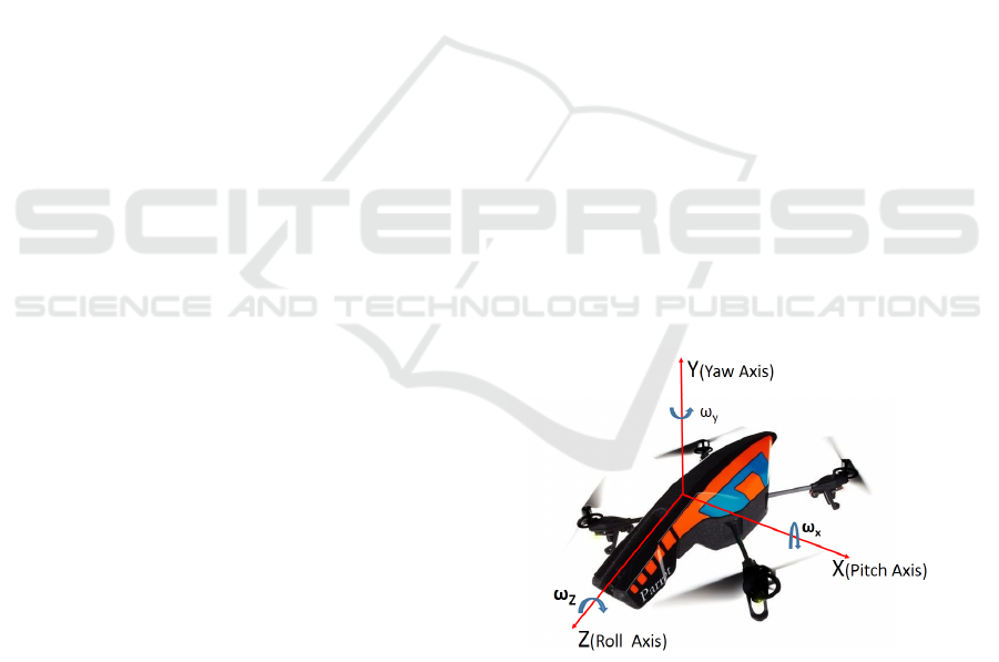
Z axis; θ, Ψ, Φ are Pitch, Roll and Yaw as shown in
Figure 1. Commonly aircraft motion estimation are
based on feature points in successive frames. Optical
flow with Horizon constraint gives the χ. (Adiv, 1985)
has reconstructed the angular velocity and linear ve-
locity of moving objects using optical flow. But their
formulation has inherent ambiguity in the noisy envi-
ronments and is based on linear optimization. (Jep-
Figure 1: Axis Convention.
son and Heegar, 1991) first calculated the translation
parameter, then using this and other information esti-
mated the rotation parameter. However there method
is liable to be unreliable if the surface is not smooth.
(Sazdovski et al., 2010) estimated the aircraft attitude
using a single on board camera. The proposed ap-
proach assumes that position of aircraft and feature
points in the camera images are known.
(Soatto et al., 1996) derived the implicit extended
Kalman filter (IEKF) for estimating displacement and
rotation that incorporates an implicit formulation into
the framework of the IEKF on the random walk
model. The IEKF implementation was applied on
the non linear space to characterize the motion of a
cloud of feature points about a fixed camera. (Grabe
et al., 2012) had use continuous homography con-
543
Abhishek A. and Venkatesh K..
UAV Autonomous Motion Estimation Methodologies.
DOI: 10.5220/0005302805430550
In Proceedings of the 10th International Conference on Computer Vision Theory and Applications (VISAPP-2015), pages 543-550
ISBN: 978-989-758-091-8
Copyright
c
 2015 SCITEPRESS (Science and Technology Publications, Lda.)

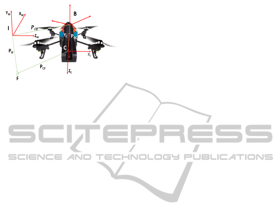
Figure 2: Relationship among Camera reference frame,
Body reference frame and Inertial frame.
straint (Ma et al., 2004) for linear velocity estimation,
integrated the result with IMU for partial state estima-
tion using computer vision. (Dusha et al., 2007) pro-
posed algorithm based on Kalman filter and optical
for state estimation. Detected lines optical flow are
tested against the motion filter. Then Kalman filter
is used to remove the outlier. Their algorithm is not
suitable for real world scenario. (Oreifej et al., 2011)
have used horizon constraint to estimate the pitch and
roll. First they had detected horizon from the image,
slope and height of the detected horizon from refer-
ence point was used for pitch and roll estimation. In
our formulation pitch and roll estimation does not re-
quire extra computations.
In Section 2 we discuss the theoretical background
of this work. Section 3 describes how the continu-
ous homography constraint is harnessed to find sys-
tem model used in Kalman filter. Section 4 discusses
the simulation results and practical considerations and
lastly concludes with Conclusion.
2 THEORETICAL BACKGROUND
2.1 System Model
Position and velocity in 3D space has meaning only if
described with respect to a frame of reference (coor-
dinate system). Depending on the requirement differ-
ent coordinate systems are used in different context.
Here, we will be dealing with camera reference frame,
body reference frame and inertial frame as shown in
Figure 2. The orientation of a general aircraft, with a
front camera is shown in this figure. The aircraft body
frame B, is fixed at the aircraft center of gravity and is
located with respect to the any inertial frame I, by the
vector P
IB
. The camera reference frame C, is fixed to
the aircraft and is located with respect to B by the vec-
tor P
BC
. The tracked features point of the environment
is denoted by F, which is located relative to I by P
IF
.
The vector P
CF
relates the relative position of F with
respect to C. These coordinate systems have differ-
ent spatial configurations, so suitable transformation
of coordinate frame is required for mapping a vector
represented in one reference frame to another refer-
ence frame. ℜ
BC
is the Euler angles transformation
relating B and C and ℜ
IB
is the Euler angles trans-
formation relating I and B. ℜ
IB
and ℜ
BC
∈ SO(3).
The mathematical relationship among them is given
in Equation 2
P
CF
= ℜ
BC
∗ ℜ
IB
(P
IB
− P
IF
) −ℜ
BC
∗ P
BC
(2)
We also assume that ground is planar. This as-
sumption is perfectly valid when UAV is at certain
height above the ground or ground surface has mi-
nor ups and downs. The Z
w
and X
w
axis of the world
frame lie on the ground plane. Negative Y
w
axis of
world frame points downward to the centre of the
earth and perpendicular to the surface of the earth.
The Z
c
axis of the camera is along the optical axis
of the camera such that Z
c
and Z
w
lie in the same
plane. The X
c
and Y
c
axis of the camera are paral-
lel to the bottom edge and the left edge of the image
plane respectively, with the origin at the optical centre
as shown in Figure 2. Any point P
w
∈ ℜ
3
in the world
frame will have the coordinate P
c
∈ ℜ
3
in the camera
frame given by
P
c
= R
c
w
P
w
(3)
where R
c
w
is the direction cosine matrix, representing
the rotation from world frame to camera frame. Let
the rigid object in the scene undergo translation T =
[T
x
, T
y
, T
z
] and small rotation Ω = [Ω
x
, Ω
y
, Ω
z
], rela-
tive to the camera. Let the object position relative to
the camera be X
t1
=[X, Y , Z] at time t1 and X
t2
= [X
2
,
Y
2
, Z
2
] at time t2, such that t2 > t1 then
X
t2
= RX
t1
+ T (4a)
R =


1 −Ω
z
Ω
y
Ω
z
1 −Ω
x
−Ω
y
Ω
x
1


(4b)
If V = [V
x
, V
y
, V
z
] is linear velocity and ω = [ω
x
,
ω
y
, ω
z
] is angular velocity, then differentiating above
equation gives the total velocity
˙
X
t1
.
˙
X
t1
=
ˆ
ωX
t1
+V (5)
where
ˆ
ω ∈ so(3) is skew symmetric matrix of ω.
2.2 Continuous Homography
Constraint
Epipolar constraint states that feature point x
1
x
1
x
1
∈ ℜ
3×1
in a frame, its corresponding location x
2
x
2
x
2
in the consec-
utive frame satisfies following constraint (Zisserman
VISAPP2015-InternationalConferenceonComputerVisionTheoryandApplications
544

and Hartley, 2004)
x
2
x
2
x
2
T
Ex
1
x
1
x
1
= 0 (6)
where E =
ˆ
T R ∈ ℜ
3×3
is known as essential matrix,
R ∈ ℜ
3×3
is rotation,
ˆ
T ∈ ℜ
3×3
is skew symmetric
matric of T . Assuming pinhole camera model, fea-
ture point X
X
X = [X,Y , Z] and its corresponding image
coordinate x
x
x = [x, y, 1] satisfy
KX
X
X = λx
x
x
where λ is unknown scale factor, K is intrinsic camera
calibration matrix. Let N ∈ ℜ
3×1
be surface normal
and d be the shortest distance of the plane from the
camera reference frame then any point X
X
X lying on the
plane satisfies
(N/d)
T
X
X
X = 1 (7)
Using above equations we have (Ma et al., 2004)
ˆx
ˆx
ˆxu
u
u = ˆx
ˆx
ˆxHx
x
x (8)
where u
u
u = [u ,v,0]
T
is optical flow, and H is the Con-
tinuous homography matrix given as
H = KHK
−1
= K(
ˆ
ω +V (N/d)
T
)K
−1
H =


h
1
h
2
h
3
h
4
h
5
h
6
h
7
h
8
h
9


(9)
3 STATE ESTIMATION
The Kalman filter is a set of mathematical equations
that provides an efficient recursive means to estimate
the state of a linear dynamic system discretized in the
time domain on the basis a of noisy measurement. It
models the state of a system at a time t
k
, as a func-
tion of the prior state at time t
k−1
, according to the
equation
x
k
= F
k
x
k−1
+ B
k
u
k
+ w
k
(10a)
z
k
= H
k
x
k
+ v
k
(10b)
where x
k
is the state vector containing, w
k
is state
noise, F
k
is the state transition matrix, z
k
is the mea-
surement vector, H
k
is the transformation matrix, u
k
is the control input, B
k
is the control input matrix and
v
k
is measurement noise. We assume the following:
E{w
k
} = E{v
k
} = 0
E{w
k
w
T
k
} = R
w
,E{v
k
v
T
k
} = R
v
Standard Time Update equations at time t = t
k
are
given below (Kalman, 1960):
x
f
k
= F
k
x
a
k−1
+ B
k
u
k
(11a)
P
f
k
= cov(x
k
− x
f
k
) = F
k
P
k−1
F
T
k
+ R
w
(11b)
x
f
k
is the predicted state at time t
k
, P
f
k
is the predicted
state covariance at time t
k
, x
a
k−1
is the estimated value
of x
k−1
and R
w
is process noise covariance. Also stan-
dard Measurement Update equations at time t = t
k
are
x
a
k
= x
f
k
+ K
k
(z
k
− H
k
x
f
k
) (12a)
P
k
= cov(x
k
− x
a
k
) = P
f
k
− K
k
H
k
P
f
k
(12b)
x
a
k
is the estimated state of x
k
and P
k
is the Posteriori
State Covariance, where innovation covariance Q and
Kalman gain K
k
are given by
Q = cov(z
k
− H
k
x
f
k
) = H
k
P
f
k
H
T
k
+ R
v
K
k
= P
f
k
H
T
k
Q
−1
We now derived a system model of UAV based on
continuous homography constraint. Putting the values
of all the parameters in Equation 8, we get
u = xh
1
+ yh
2
+ h
3
− x
2
h
7
− xyh
8
− xh
9
(13a)
v = xh
4
+ yh
5
+ h
6
− xyh
7
− y
2
h
8
− yh
9
(13b)
−yu + xv = −xyh
1
+ x
2
h
4
− y
2
h
2
+ xyh
5
− yh
3
+ xh
6
(13c)
Multiplying Equation 13a by −y and Equation 13b by
x on both sides yields Equation 13c. Therefore, it is a
dependent set of equations, and only top two of them
are used for estimating H. Above system model is lin-
ear w.r.t [h
1
,h
2
,...h
9
] but they are nonlinear on Con-
tinuous homography space H . H belongs to a subset
of ℜ
3×3
whose eigen values possess unique charac-
teristics. Taken any random value of ω, N and V as
given below
ω =

41 13 47

N =

31 24 18

V =

18 10 13

Without the loss of generality assuming d = 1 then
H =


558 385 337
357 240 139
390 353 234


The eigen values λ of H + H
T
are
(2082.5,0,−18.51). λ
1
> 0, λ
2
= 0 and λ
3
<
0. This is true for any H which belongs to the
continuous homography group H . So after solving
Equations 13a and 13b for [h
1
,h
2
,...h
9
], it will be
projected to space H . Let h
k
be the state vector and
z
k
the measurement vector at time t = t
k
h
k
=

h
1
h
2
h
3
h
4
h
5
h
6
h
7
h
8
h
9

T
z
k
=

x y u v

T
UAVAutonomousMotionEstimationMethodologies
545

Rewriting Equations 13a and 13b in implicit form
gives

x y 1 0 0 0 −x
2
−xy −x
0 0 0 x y 1 −xy −y
2
−y

| {z }
ζ
k
h
k
+

−u
−v

| {z }
U
k
= 0 (14)
Denote above equation by g(h
k
,z
k
). Assuming h
k
and
z
k
are slowly varying, they can be modeled as
h
k
= f (h
k−1
) +w
k
;w
k
∈ N (0,R
w
) (15)
z
k
= z
t
k
+ v
k
;v
k
∈ N (0,R
v
) (16)
where f ( ) is nonlinear vector functions and z
t
k
is true
value of z
k
. Linearising Equation 15 at time t
k
using
previous estimate h
a
k−1
, we get
h
k
≈ f (h
a
k−1
) + J
f
(h
a
k−1
)(h
k−1
− h
a
k−1
) + w
k
+ H.O.T
where J
f
is Jacobian of function f w.r.t h
k
. We as-
sume that all h
k
is very close to h
a
k−1
, so higher order
terms can be ignored. Rewriting this in form as given
in equation 10
h
k
≈ F
k
h
k−1
+ u
k
+ w
k
(17)
where
F
k
= J
f
(h
a
k−1
)
u
k
= f (h
a
k−1
) −J
f
(h
a
k−1
)h
a
k−1
Therefore predicated value of h
k
, h
f
k
is given by
h
f
k
= F
k
h
a
k−1
+ u
k
= J
f
(h
a
k−1
)h
a
k−1
+ f (h
a
k−1
) −J
f
(h
a
k−1
)h
a
k−1
= f (h
a
k−1
) (18)
Similarly Predicted state covariance P
f
k
is
P
f
k
= J
f
(h
a
k−1
)P
k−1
J
f
(h
a
k−1
)
T
+ R
w
(19)
Linearising the g(h
k
,z
k
) about (h
f
k
,z
t
k
) results,
g(h
k
,z
k
) ≈ g(h
f
k
,z
t
k
) + J
h
(h
f
k
)(h
k
− h
f
k
) + J
z
(z
t
k
)(z
k
− z
t
k
)
where J
h
is Jacobian of g(h
k
,z
k
) w.r.t h
k
and J
z
is Jaco-
bian of g(h
k
,z
k
) w.r.t z
k
. But, g(h
k
,z
k
) = 0 and z
k
− z
t
k
= v
k
. Rearranging the equation in Standard form
−g(h
f
k
,z
t
k
) +J
h
(h
f
k
)h
f
k
= J
h
(h
f
k
)h
k
+ J
z
(z
t
k
)v
k
⇒ ˜g(h
k
,z
k
) = H
k
h
k
+ ˜v
k
Comparing this with equation 10, measurement up-
date equations are
h
a
k
= h
f
k
+ K
k
( ˜g(h
f
k
,z
k
) −H
k
h
f
k
)
= h
f
k
− K
k
(ζ
k
h
k
+ U
k
) (20)
P
k
= P
f
k
− K
k
ζ
k
P
f
k
(21)
Algorithm 1: State estimation using Kalman Filter.
Given set of n feature points and optical flow, find (ω,
V ), pitch and roll
1: Initialisation of State Variable
Form the equations as mentioned in the Equations
13a and 13b. Solve for h and stack it to form H.
Normalize H to find H = H −
e
2
2
I. Estimate the
initial error covariance P
0
and h
f
0
.
2: Time update
Predict the current state of system on the basis of
previous estimate.
h
f
k
= h
a
k−1
P
f
k
= P
k−1
+ R
w
3: Measurement Update
Estimate the best current state using time update
results.
h
a
k
= h
f
k
- K
k
(ζh + U)
P
k
= P
f
k
− K
k
J
h
(h
f
k
)P
f
k
Above equation will be solved as follows
• Compute square root of P
f
k
,
´
R
v
using LDL
T
.
• Form the block matrix, O is zero matrix.
pre =
´
R
v
T /2
O
P
f T /2
k
ζ
T
P
f T /2
k
!
• QR factorization of above will result in
post =
Q
T /2
Q
−1/2
ζP
f
k
O
T
P
T /2
k
!
• P
k
= post(end − k : end,end − k : end) where
end is number of rows and k is number of state
vector.
• Similarly solve for other equations..
4: Projection on Continuous homography space
Stack h
k
to get H and normalize it to obtain H.
5: Recover State
Decompose H to estimate V , N and ω (Ma et al.,
2004).
Using N estimate pitch and roll.
where
K
k
= P
f
k
ζ
T
k
Q
−1
Q = ζ
k
P
f
k
ζ
T
k
+
´
R
v
´
R
v
= J
z
(z
t
k
)R
v
J
T
z
(z
t
k
)
where T denotes the transpose of matrix. h
k
found
in above equations generally will not belong to H .
Hence h
k
will be projected on to H . For this stack
the [h
1
,h
2
,...h
9
] to form H∈ℜ
3×3
. The continuous
homography matrix H is given by
H = H −
e
2
2
I (22)
VISAPP2015-InternationalConferenceonComputerVisionTheoryandApplications
546

where I is identity matrix and e
2
is second largest
eigenvalue of H +H
T
. Once H is known, (ω, V ) is es-
timated using steps mentioned in Algorithm 1. Now
we will show procedure for pitch and roll estimation
from N. Given axis convention in Figure 2, unit nor-
mal to the ground is
´
N = [0,1,0]. Due to different ori-
entation of coordinate axes
´
N will appear as N from
the reference frame B, relation among them is given
by Equation3, R
c
w
is given by
R
c
w
=


cosΦ 0 sinΦ
0 1 0
−sin Φ 0 cos Φ




1 0 0
0 cos θ − sinθ
0 sinθ cos θ




cosΨ −sin Ψ 0
sinΨ cos Ψ 0
0 0 1


N is independent of yaw and translation, hence solv-
ing for N yields
N = [−sinΨ, cos Ψ cos θ, cos Ψ sin θ]
T
(23)
Pitch θ and roll Ψ are calculated from N using rela-
tions given below
Ψ =
arccos
q
N
2
2
+ N
2
3
+ arcsinN
1
2
(24)
θ =
arccos
N
2
cosΨ
+ arcsin
N
3
cosΨ
2
(25)
Above method for calculating pitch and roll depends
only on feature points implying these can be esti-
mated in wide range of environment opposed horizon
constraint based methods.
Theocratically, P
k
is symmetric positive definite,
but numerical implementation sometimes led to P
k
that became nonsymmetric and/or indefinite. The sit-
uation becomes worse if the matrix dimensions are
large. Thus, to improve the condition number, and
hence the numerical stability to the noise, square root
filter is used. Square root filtering implementation
provides twice the precision than standard kalman fil-
ter implementation. Cholesky factorization is used to
find the square root of positive definite matrix. In
practice, however, the estimation problems are severe
as some outliers can seriously pollute the sample, thus
making the matrix non positive definite. To avoid this
issue, LDL
T
factorization is used. The LDL
T
factor-
ization uniquely factors the symmetric matrix P as
P = LDL
T
where L is a lower triangular matrix with 1 as diag-
onal element, D is a diagonal matrix. It is more ef-
ficient than Cholesky factorization because it avoids
computing the square roots of the diagonal elements
and is always stable. Due to noise some insignificant
eigenvalues are neglected. From LDL
T
, the Cholesky
factorization will be computed as follows
P = LDL
T
= (LD
1/2
)(D
1/2
L) (26)
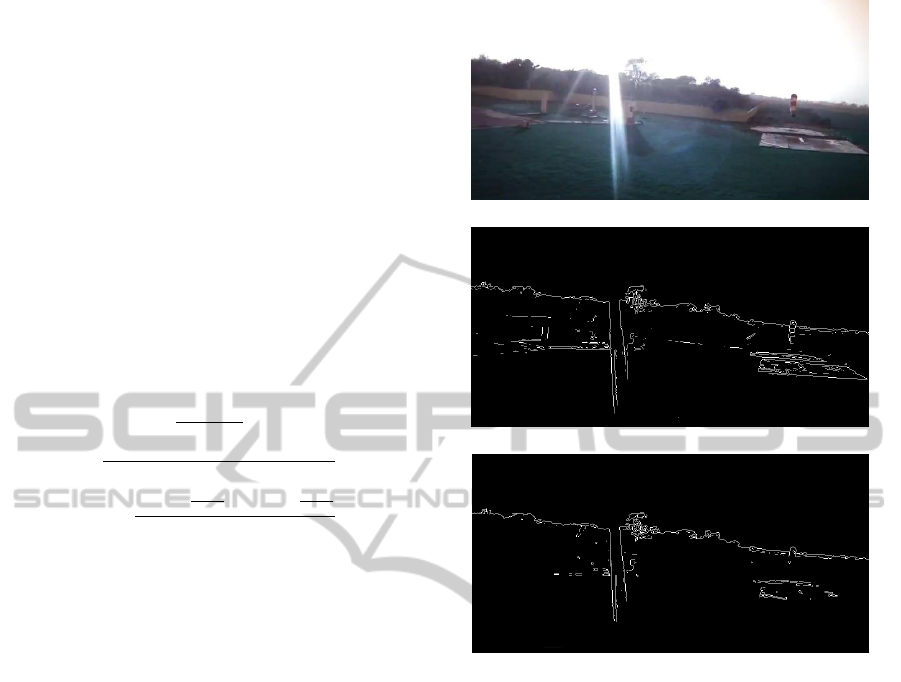
(a) RGB image
(b) Edge Map
(c) Edge map using Equation 27
Figure 3: Edge map comparison using different color to
grayscale conversion relations.
4 SIMULATION RESULTS
Multiple experiments were conducted on outdoor en-
vironment using Parrot AR Drone shown in Fig-
ure 1, for the verification of algorithms proposed in
this discussion. The algorithms were tested on both
OpenCv and Matlab platforms. We have used Par-
rot AR Drone SDK for capturing video(30 frame per
second) and IMU data.
For converting RGB to grayscale we have used
Equation 27. We found that feature tracking gives
better results when following relation is used for con-
verting RGB image to grayscale image.
GS = min(min(255 − R, 255 − G),255 − B) (27)
where R, G and B are red, green and blue color chan-
nel of an RGB image, and GS is grayscale image. This
conversion removes the noise and makes feature de-
tection more robust than other grayscale conversion
methods. Figure 3(a) shows a frame captured by the
UAVAutonomousMotionEstimationMethodologies
547

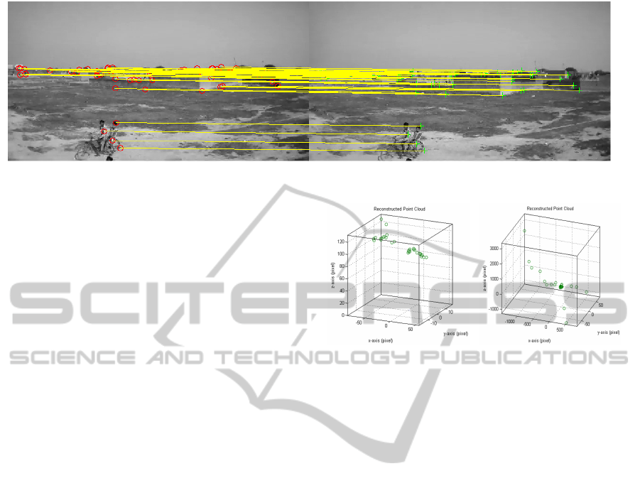
Figure 4: Feature points extraction and matching.
UAV. Due to the large height of UAV from the ground,
the image transmitted over Wifi to the ground station,
is not of a good quality and has poor contrast. Edge
map of the corresponding image using Matlab inbuilt
RGB to grayscale conversion is shown in Figure 3(b).
The edge map has a large number of false and stray
edges due to the poor quality of image and the pres-
ence of noise. The strong edges, caused due to sun-
light are also undesired. In Figure 3(c), a large num-
ber of false edges are removed using relation men-
tioned in Equation 27. Feature points are the points
of interest in an image. Most commonly used fea-
tures are the edges and corners. We have used Har-
ris corner descriptor for feature extraction and track-
ing. The Harris corner detector is a commonly used
interest point detector, owing to its strong invariance
to scale, rotation, image noise and illumination vari-
ation(Schmid et al., 2000). Correspondence based
technique is used for feature tracking between frames.
Correspondence based techniques extract a set of fea-
tures from each frame, and then attempt to estab-
lish correspondences between consecutive sets of fea-
tures. To deal with large motion hierarchical search
strategy is used. The patches in consecutive frames
are compared using a translational model, and then
these location estimates are used to initialize an affine
registration between the patch in the current frame
and the base frame, where a feature was first de-
tected(Shi and Tomasi, 1994). Also number of fea-
tures point used for correspondence between consec-
utive images depends on type of environment.
4.1 ω and V Estimation
Various methodologies for state estimation were
adopted in experiments, to find harmony between the
theoretical concepts and the actual output of the sen-
sor. States are estimated solving Continuous homog-
raphy constraint for each frame and approach dis-
cussed above. Most of above mentioned algorithms
give multiple solutions for linear and angular veloc-
ity. This inherent ambiguity is removed using positive
(a) Configuration 1 (b) Configuration 2
Figure 5: 3D point reconstruction.
depth constraint. Here, we first show the results of 3D
reconstruction, and then state estimation, followed by
a comparison among them.
We have reconstructed the 3D point from the cam-
era matrix obtained in our experiment. Figure 5,
shows the two possible orientation of the 3D points
with respect to camera, reconstructed from feature
points extracted from frame taken by our UAV as
shown in Figure 4. Other two possible 3D recon-
structed points are mirror image of Figure 5(a) and
5(b) respectively. It is difficult to visualise the above
point coordinates in 3D, thus the projection of Con-
figuration 1 on X , Y , Z plane is shown in Figure 6.
These points have been scaled with a scale factor of
100 (randomly selected), as the reconstructed points
are obtained upto a scale factor. These reconstructed
points have both positive and negative X and Y co-
ordinates but always have positive depth i.e all have
a positive Z coordinate, i.e the assumption we have
taken about the body coordinate system(Refer to Fig-
ure 2). The other configuration is just a mirror image.
Similarly, the projection of Configuration 2 on X, Y ,
Z plane is shown in Figure 7. Reconstructed points
are spread along both positive and negative axis. The
other configuration will the mirror image. Among
these only Configuration 1 is valid justifying our as-
sumption. This result also supports validity of com-
puter vision approach for state estimation.
The angular velocity estimated from various al-
gorithms is shown in Figure 8, where IMU stands
VISAPP2015-InternationalConferenceonComputerVisionTheoryandApplications
548

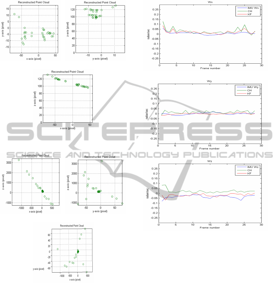
(a) Projection on X −Y (b) Projection on Y − Z
(c) Projection on Z − X
Figure 6: Configuration 1.
(a) Projection on X −Z (b) Projection on Y − Z
(c) Projection on X −Y
Figure 7: Configuration 2.
for measurement obtained form Inertial measurement
unit, CH stands for Continuous homography con-
straint and KF stands for Implicit square root kalman
filter. Angular velocity i.e ω
x
, ω
y
, ω
z
estimated using
these method approximately follows the IMU.
The linear velocity is also estimated using all the
above mentioned methods. But, in the absence of any
3D information, it can be estimated only upto a scale
factor. Implicit square root kalman filter based algo-
rithm gives the better result than continuous homog-
raphy based method.
(a) About X axis
(b) About Y axis
(c) About Z axis
Figure 8: ω estimation.
4.2 Pitch and Roll Estimation
Pitch and roll estimated using horizon constraint(HC)
is shown in the Figure 9. Pitch estimation is more
prone to error than roll estimation using horizon con-
straint. Because pitch estimation depends on the
height while roll depends on the slope of detected
horizon line. Pitch estimation is only accurate if
the constant height assumption is valid. If horizon
is not present, then pitch and roll cannot be found.
There are no such limitations in continuous homog-
raphy constraint based algorithm (shown as CH in
the plot). Figure 9 shows the comparison among
them with ground truth. In our experiments Implicit
square root kalman filter based algorithm proved to
be more promising than horizon constraint based ap-
proach, because it solely depends upon the feature
points. Proposed method can be used in any environ-
UAVAutonomousMotionEstimationMethodologies
549

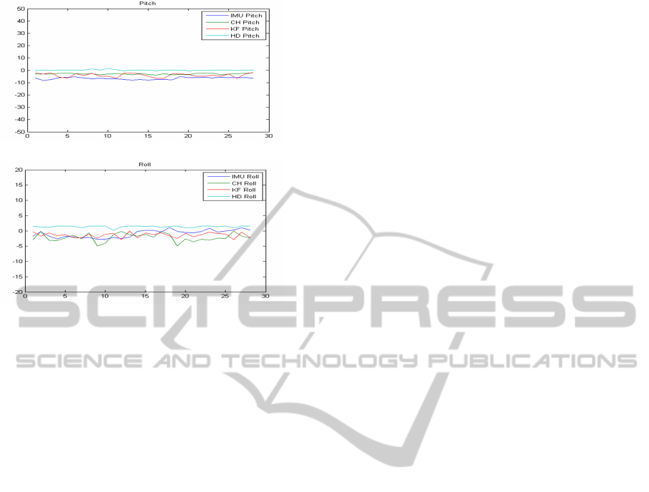
(a) Pitch
(b) Roll
Figure 9: Pitch and Roll Estimation.
ment provided sufficient number of features points are
available.
5 CONCLUSIONS
Computer vision based approaches are attractive due
to low weight, low cost and existing presence of a
camera on the vehicle. This work gives an insight
into the application of onboard cameras for state esti-
mation, without using any additional sensors. Linear
and angular velocity estimation algorithm has been
developed using implicit extended Kalman filter. We
have removed the horizon constraint in the estima-
tion of pitch and roll. They can be estimated more
accurately without any horizon constraint. Also fea-
ture points correspondence are required for calculat-
ing sparse optical flow, so pitch and roll estimation
do not require extra processing as opposed to horizon
constraint where horizon line segment is required for
finding these parameters. The results clearly manifest
the feasibility of algorithms for real time applications.
Although the results are inspiring, yet these ap-
proaches are limited to an environment where suffi-
cient feature points are available. It cannot be used if
a good number of feature points is not available. Also
we have assumed planar surface, this assumption is
not valid if UAV is closer to earth surface. This work
can be extended to environment were less number of
features points are available and earth surface has un-
even ups and downs. We have assumed that a camera
is fixed to the UAV, which can be relaxed with little
complexity, so that the camera may always point to-
wards the region where a sufficient number of feature
points are available. Further computation complexity
can be reduced. Finally, this work is based on RGB
camera which is highly sensitive to lighting condition,
and thus developing a system based on the IR camera
would be beneficial because that will enable its use
even in low lighting conditions.
REFERENCES
Adiv, G. (July 1985). Determining three-dimensional mo-
tion and structure from optical flow generated by sev-
eral moving objects. IEEE Transactions on pattern
analysis and machine intelligence, 7(4):384 – 401.
Dusha, D., Boles, W., and Walker, R. (Dec. 2007). Atti-
tude estimation for a fixed-wing aircraft using horizon
detection and optical flow. In Digital Image Comput-
ing Techniques and Applications, Australian Pattern
Recognition Society on, pages 485 – 492.
Grabe, V., Bulthoff, H., and Giordano, P. (2012). On-
board velocity estimation and closed-loop control of
a quadrotor uav based on optical flow. In IEEE Inter-
national Conference on, pages 491–497.
Jepson, A. D. and Heegar, D. J. (1991). A fast subspace
algorithm for recovering rigid motion. In Visual Mo-
tion, Proceedings of the IEEE Workshop on, pages 124
– 131.
Kalman, R. E. (1960). A new approach to linear filtering
and prediction problems. 82:35–45.
Ma, Y., Soatto, S., Kosecka, J., and Sastry, S. (2004). An
Invitation to 3-D Vision: From Images to Geometric
Models. Springer.
Oreifej, O., Lobo, N., and Shah, M. (2011). Horizon
constraint for unambiguous uav navigation in planar
scenes. In Robotics and Automation (ICRA), 2011
IEEE International Conference on, pages 1159–1165.
Sazdovski, V., Silson, P., and Tsourdos, A. (2010). Atti-
tude determination from single camera vector obser-
vations. In Intelligent Systems (IS), 2010 5th IEEE
International Conference, pages 49–54.
Schmid, C., Mohr, R., and Bauckhage, C. (June 2000).
Evaluation of interest point detectors. International
Journal of Computer Vision, 37(2):151–172.
Shi, J. and Tomasi, C. (June 1994). Good features to track.
In Computer Vision and Pattern Recognition,IEEE
Computer Society Conference on, pages 593–600.
Siouris, G. M. (1993). Aerospace Avionics Systems : A
Modern Synthesis. Academic Press Inc.
Soatto, S., Frezza, R., and Perona, P. (March 1996). Mo-
tion estimation via dynamic vision. Automatic Con-
trol, IEEE Transactions on, 4(3):393–413.
Zisserman, A. and Hartley, R. (2004). Multiple View Geom-
etry in Computer Vision. Cambridge University Press.
VISAPP2015-InternationalConferenceonComputerVisionTheoryandApplications
550