Adaptive Segmentation by Combinatorial Optimization

Lakhdar Grouche and Aissa Belmeguenai

Laboratoire de Recherche en Electronique de Skikda LRES, 20 aoˆut University, BP 26 Route El Hadaeik, Skikda, Algeria

Keywords:

Iterative Segmentation, Kangaroo Method, Non-oriented Graph, Entire Number Formulation, Combinatorial

Optimization.

Abstract:

In this paper we present an iterative segmentation. At the beginning it is using a stochastic method called

Kangaroo in order to speed up the regions construction. Later the problem will be presented as non-oriented

graph then reconstructed by linear software as entire number. Next, we use the combinatorial optimization to

solve the system into entire number.

Finally, the impact of this solution became apparent by segmentation, in which the edges are marked with

special manner; hence the results are very encouraging.

1 INTRODUCTION

The techniques of images segmentation have seen

considerable development these last years, because

we have passed the split-and-merge (H.Yang, 1997),

to the use of watersheds, to active edges mini-

mization, and ﬁnally to multi-agents segmentation

(S.Mazouzi, 2007).

The segmentation methods by increasing regions

based to measurement relatedto gray level,or to prob-

ability measurement, bring a good initial identiﬁca-

tion for regions of interest, but suffer from the ma-

jor inconvenient of non precise localization of regions

edges. The approach of segmentation by the active

edges presents good results concerning the localiza-

tion of regions edges of interest, providing that the

initialization of these edges will not be far from the

ﬁnal edges. The hybrid approaches can combine in-

formation coming from several methods looking very

promising.

These diversitiesof methods have made that we do

not have a universal method of segmentation, but we

have an algorithm of segmentation to be used for each

application and its evaluation depends on the obtained

results. This complexity is related to the principle of

segmentation, because we are looking for a compro-

mise between an over segmentation in which there are

so much details and an under segmentation in which

there are a lack of details (W.Eziddin, 2012).

Finally, as a conclusion of the image method seg-

mentation, we can underline that the iterative method

of segmentation lead, in general, to the best results

than the non-iterative methods.

In the present work we have developed an iterative

method of segmentation, which treat directly the com-

promise of segmentation, it is intended performance

by the following strengths:

1. Self adaptive: it does adapt automatically with the

sample in order to avoid huge number of iteration.

This self-adaptive sentence will be constituted of

two other sentences:

(a) One ﬁrst sentence in which we have used a

heuristic to estimate the step used during the

constitution of regions, in order to reduce the

number of iteration and consequently the exe-

cution time of this sentence.

(b) A second sentence which is of practical use,

this heuristic will be applied on images of dif-

ferent nature, in which the gray level inside

each region is almost constant, more or less

constant and completely variable.

2. Optimal: the problem formulation as entire then

the use of the graphs theory and the combina-

torial optimization enable the ﬁne segmentation

and avoid the oversegmentation or the under-

segmentation.

Its application on diversity of samples, contain at the

same time regions of close levels, and regions of too

far levels, givinggood results. By this fact our method

turns effective, and it is valid for a large variety of

applications.

Grouche L. and Belmeguenai A..

Adaptive Segmentation by Combinatorial Optimization.

DOI: 10.5220/0005301300920097

In Proceedings of the 10th International Conference on Computer Vision Theory and Applications (VISAPP-2015), pages 92-97

ISBN: 978-989-758-089-5

 2015 SCITEPRESS (Science and Technology Publications, Lda.)

2 THEORETICAL TOOLS

2.1 Deﬁnitions

The segmentation of an image A, regarding the ho-

mogenous criteria H (gray level, texture,..) , is a par-

tition of A on homogenous regions r

, r

, . . . , r

H have an argument for one or several regions close

to the initial image A to return a decision of its homo-

geneity, H((r

, r

, ...) ∈ Z

) → {true, false}. In our

work, we introduce several parameters on the region

that we would like to study, these latter will be devel-

oped in the section 2.3.

[

i=1

) = A (1)

∀i ∈ {1, 2, . . . , n} r

is related (2)

∀i ∈ {1, 2, . . . , n} H(r

) is true (3)

∀r

, r

voisines H(r

, r

) is false. (4)

Regarding this deﬁnition, the segmentation depends

on the criteria H used. The choice of this criterion is

really primordial.

2.2 Regions Training

Let A the image to make segmentation with a(i, j),

the gray level of pixels and C the image label (the im-

age of labeled regions) with c(i, j), the gray level of

pixels, the pixels of each region have the same level

noted code. To go from A to C, we proceed with dou-

ble scan as follow. Each pixel c(i, j) ∈ C is computed

by the Algorithm Code.

Algorithm Code

Initialization: we initialize the code = 1, the gap ε =

0, we start with the pixel high-left of the image

c(1, 1) = code.

Horizontal: for two horizontal pixels close:

If |a(i, j) − a(i, j + 1)| ≤ ε

then c(i, j + 1) = c(i, j)

else code = code+ 1 , c(i, j + 1) = code;

EndIf

If (end of line)

then code = code+ 1

EndIf

Vertical: for two vertical pixels close:

If (|a(i, j) − a(i+ 1, j)| ≤ ε) then

c(i, j) = min(c(i, j), c(i+ 1, j))

c(i+ 1, j) = min(c(i, j), c(i+ 1, j));

EndIf

Equality: Iterate the vertical scan untill not equality

of image C.

Let B the vector of codes used in the Algorithm Code

so lentgh(B) = n.

A propagation with equality levels ε = 0 give

regions only for perfect images, but in the general

case the levels of the same region are variables,

they vary from one sample to the other. So we

have to make compromise between one ε weak giv-

ing over-segmentation and another big giving under-

segmentation. To this stage two approaches are pos-

sible:

1. The ﬁrst approach consists of starting from the

equality ε = 0, then increment it gradually, till the

regions training, but this procedure is boring in

time, because the propagation process is repeated

each iteration. This drawback is appearing usually

for far regions levels.

2. A second approach consists of starting from the

equality ε = 0, then ﬁnd an estimation function

which adapt the increment step according to the

sample. This self adaption increase the quickly

the step ε, decrease the number of iteration and

speed up the convergenceprocess to regions train-

ing. A detailed method of speed up will be pre-

sented in section 3.1 .

Finally the two approaches require a stop condition;

this latter is ﬁxed according to the classiﬁcation rate

of pixels in regions.

2.3 Connection Graph

Having A, C and B, we proceed to the regions extrac-

tion one by one. For each region, we determine the

following parameters (A.Herbulot, 2007); for exam-

ple for one region r

coded by B(i),

• s

the surface of r

• µ

the average level,

• h

the histogram,

• ρ

= {x : h

(x) = max(h

)} the mode,

• I

= [a, b] such as Σ

x=a

(x) > 0.8 ∗ Σ

255

x=0

(x)

the conﬁdence interval .

The coded image C leads to non oriented graph G =

(V, E) (E.Fleury, 2009; F.Khadar, 2009).

AdaptiveSegmentationbyCombinatorialOptimization

- The set of nodes V present the regions r

with i ∈

V (1) in which each node is characterized by its

parameters (s

, µ

, h

, ρ

, I

) and kVk = n.

- A link between i and j, e = (i, j) ∈ E such as i, j ∈

V show the regions r

and r

are close. This link

does not exist unless the parameters of regions are

distinct (3) and (4).

3 PROBLEM FORMULATION

3.1 The Kangaroo Method to Speed up

the Convergence

The stochastic method of Kangaroo (G.Fleury, 1993)

, is metaheuristic used in the NP-difﬁcult problems,

that we have adopted to our problem to accelerate the

process of regions constitutions. As indicated by its

name, it has a variable step, thus we have experimen-

tally used an empiric formula to update the step of

each iteration (5, 6). Following the step of propaga-

tion, the trained regions of some pixels form an over-

segmentation and their pixels are not classiﬁed.

Let ψ the pixel number non classiﬁed and S = size,

the ratio of non classiﬁcation τ is expressed as:

τ =

(5)

Since this ratio is expressing the number of non-

classiﬁed pixels, so it does show good sign of the in-

crement step of Kangaroo and consequently the esti-

mation function ε. Because a high τ means that the

majority of pixels are not classiﬁed, which means that

we are far from the convergence, so we have to in-

crement the step ε and inversely for low τ means that

the process of propagation is close to the convergence,

consequently we have to reduce the step ε. In practice

several estimation functions of this step of increment

ε have been tested we have kept the one given by (6).

ε = ε+ 10.τ (6)

The regions construction is estimated achieved when

τ < 10%, the non-classiﬁed left pixels are assigned to

the close region.

3.2 Individual Regions Processing

Now as the regions are marked, each region is ex-

tracted separately, and their parameters µ

, ρ

and

they are calculated. Then the two next logical vari-

ables are deduced:

1 if |µ

−ρ

|<s1

0 otherwise

(7)

1 if I

<s2

0 otherwise

(8)

Practically we have ﬁxed the parameters, s1 = 9, in

order that the statistical average and the region mode

are close, so signiﬁcant and s2 = 30, so that the pixels

of the same region will have a uniform visual aspect,

because beyond the human eye can make differences.

The edge e = (i, j) ∈ E will be presented by a log-

ical variable x

= x

this latter at the time of segmen-

tation optimization.

1 if r

6=r

0 otherwise

(9)

3.3 Formulation of the Problem into

Entire Number

Following the regions construction, according to

(G.L.Nemhauser and L.A.Wolsey, 1988; M.Baiou

and F.Barahona, 2011), we have the following con-

straint :

Region: each region i give two logical variables, y

and z

such as:

+ z

≥ 0 (10)

The region i is not effective unless y

+ z

= 2.

Edge: e = (i, j) ∈ E between the regions i and j pre-

sented by the variable x

= x

is not effective un-

less the regions i and j are also so. Therefore it

should verify the following constraints:











≥ 0 (false)

≤ 1 (true)

≤ y

+ y

(modes)

≤ z

+ z

(distributions)

Estimation: to have effective differences,

Maximize Σ

kVk

i=1

+ z

) (11)

Relaxation: each region i having y

+ z

< 2, it is

decomposed into two regions u and v such as

+ z

≥ 1 and y

+ z

≥ 1, then we refresh the

parameters of the graph G = (V, E) and ﬁnally

we rewrite the corresponding constraints to the re-

cently created or modiﬁed regions.

4 SEGMENTATION ALGORITHM

Our algorithm of segmentation uses the principle of

top-down iterative cutting. Having the image to be

segmented A, we proceed as follow:

VISAPP2015-InternationalConferenceonComputerVisionTheoryandApplications

i- Regions construction:

Let A the image to be segmented and C the

image of the coded regions. We denote C =

SPPpropag(A, ε) the routine enabling this code

with an error gap ε within the gray levels of the

same regions, we have used the Kangaroo method

as follow:

1 - Initialization ε = 1

2 - C = SPPpropag(A, ε)

3 - Calculation of τ then ε = ε+ Round(10.τ)

4 - If τ > 0.1

then back to the step 2

Endif

The use of this stochastic algorithm, has allowed

us to reduce with considerable manner the num-

ber of iteration of the propagation regardless the

image sample.

ii - The graph calculation :

Starting from the image of the regions code C, the

one of the departure A, a graph G = (V, E) is being

calculated. The logical variables y

, z

of each re-

gion are calculated as well as the variables edges

with a number of regions kVk.

iii - Estimation :

calculation of the combinatorial optimization

function H = Σ

kVk

i=1

+ z

If H is maximum

then end of process

else following the step of relaxation

Endif

iv - Relaxation :

for each region i having y

+ z

< 2, an optimum

cutting (K.Chehdi, 1991) is applied to decompose

this region into two sub-regions r

= r

+ r

then

back to the step ii−.

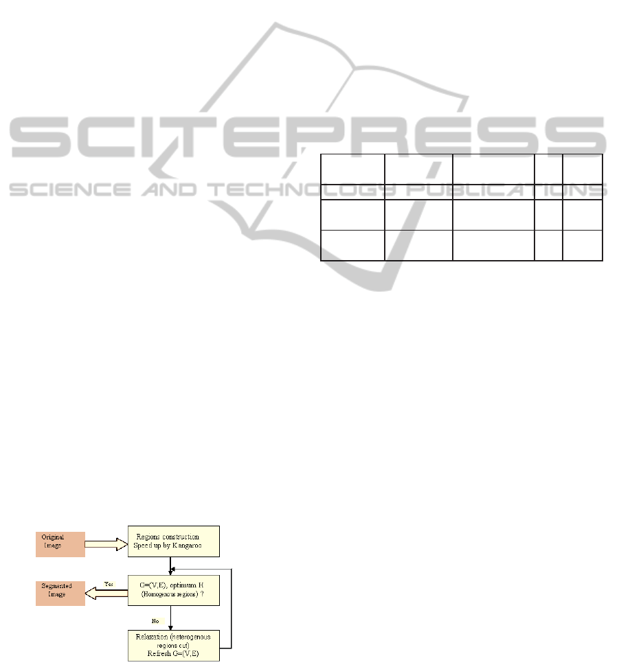
The synoptic of ﬁgure 1 summarize the steps of

our algorithm of segmentation.

Figure 1: the principle of the algorithm of segmentation.

5 EXPERIMENTAL RESULTS

5.1 Speed up the Regions Construction

By applying our method upon several images sam-

ples, we recorded the following results:

We proposed in this paper, the acceleration results

of regions which are constituted by three images in

which, the gray levels by region are homogenous

in the ﬁrst ones (Gap ≤ 4), more or less variables

(6 ≤ Gap ≤ 9) in the second and completely hetero-

geneous (25 ≤ Gap ≤ 40) in the third one.

The algorithm starts the ﬁrst iteration with a gap ε = 1

and τ is evaluated at the end of iteration according to

(5) , if the stop condition 3.1 is not reached then ε is

calculated according to (6) to start the following iter-

ation.

Table 1: Result of speed up convergence.

images Gap in Iteration of ε τ

the region SPPpropag in %

circles ≤ 4 1st iteration 1 6.6

alumgrns 6, 9 1st iteration 1 12.9

2nd iteartion 2 8.6

rice 25, 40 1st iteration 1 98

2nd iteartion 11 7.5

The results gathered in (Table 1) conﬁrm the fol-

lowing:

• The ﬁrst is indeed concerning the Kangoroo

method, because the regions constitution is al-

ways achieved in about two or three iteration,

which reduce and minimize greatly the time of

this stage.

• The second shows that our empiric formula of

Kangaroo step of evaluation ε is valid for large

range of images samples.

• The column of step ε shows that this latter varies

with respect to gray level variation inside the re-

gions, and it adapts automatically for each situa-

tion.

The gaps in gray level inside the same image, they are

variable from one region to the other. Sometimes the

regions construction which the gap is high, they will

be followed with fusion of close regions. This phe-

nomenon is totally normal because it is the Kangaroo

principle but it will be solved in the relaxation stage

which will be discussed in section 5.2 in page 5.

AdaptiveSegmentationbyCombinatorialOptimization

5.2 Relaxation and Correction of

Segmentation

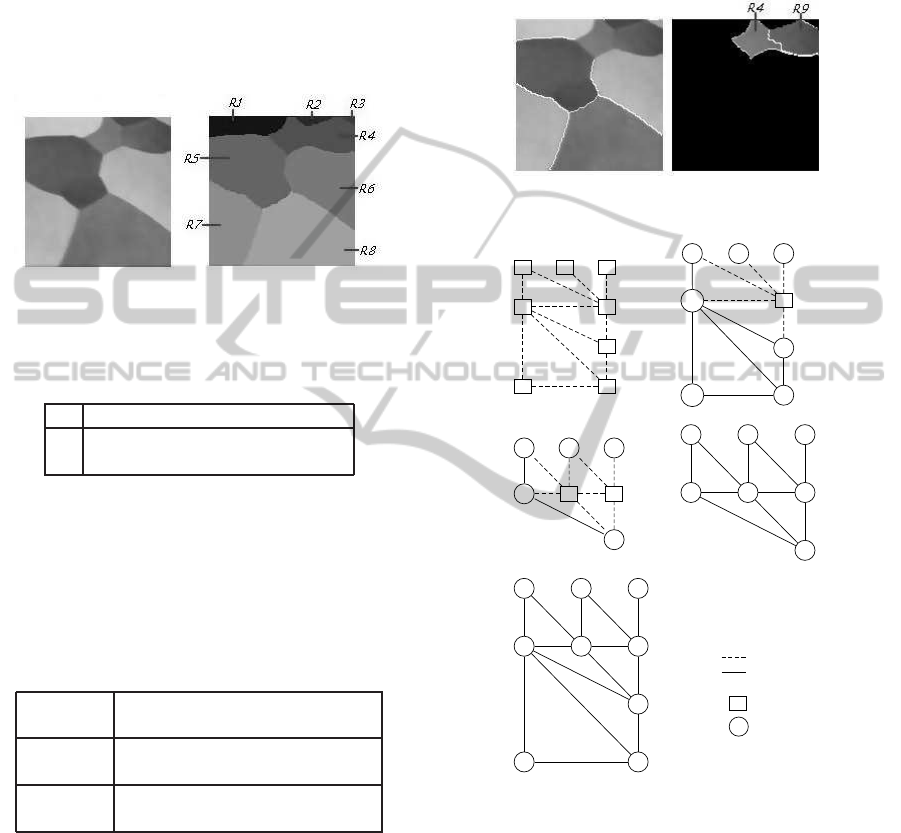
In the image of ﬁgure 2 in the left, the steps i− and

ii− of the algorithm has given the images of ﬁgure 2

in the right, presented by the graph of ﬁgure 4, high

left. This latter contain 8 regions and 11 edges, so we

have a graph G = (E,V) with kVk = 8 and kEk = 11,

having the data as follow:

Figure 2: original (left) regions (right).

The step iii− of the Algorithm has given:

Table 2: Result of the 1st iteration.

V 1 2 3 4 5 6 7 8

1 1 1 0 1 1 1 1

Thus the Table 2 illustrates the results of the ﬁrst it-

eration and as we can notice, the region r

does not

satisfy the H criteria.

a- An estimation function H = 14, whereas it’s max-

imum have to be 16, therefore it is not optimum.

b- Edges vector E, such as:

Table 3: Link vector E after the 1st estimation.

(i, j) ∈ E (1, 4) (2, 4) (3, 4) (1, 5)

0 0 0 1

(i, j) ∈ E (4, 5) (4, 6) (5, 6) (5, 7)

0 0 1 1

(i, j) ∈ E (5, 8) (6, 8) (7, 8)

1 1 1

The compounds to 0 in E correspond to missing

edges in the graph and this means that the separa-

tion between regions in these positions is not ef-

fective. Whereas the compounds to 1 correspond

to available edges in the graph and they are pre-

sented in the image by white line separating the

regions in these positions as shown by ﬁgure 3 in

left.

According to ( 9), the Table 3 shows that all the

binary variables x

connected to r

are 0 (∀(i = 4

or j = 4) ⇒ x

= 0).

c- The results of this ﬁrst iteration of estimation are

presented by the graph of ﬁgure 4 high right.

The algorithm then follows the step iv−. Regarding

the data, the relaxation acts on the region r

, because

it is the less homogenous.

Figure 3: Before the relaxation (left) after the relaxation

(right).

i j

= 0

i j

= 1

+ z

≺ 2

+ z

= 2

ÄÒ

Figure 4: Algorithm in graphs.

As we can notice, the region r

is treated sepa-

rately; the result is illustrated by ﬁgure 3 left. This

step of relaxation is illustrated by the graph of ﬁgure

4 down left. It has lead to two new regions rated 4 and

9, having the parameters y

= z

= 1, and y

= z

= 1.

Following this stage, the second iteration of es-

timation gives new graph G = (E,V), presented by

ﬁgure 4 down right, such as kVk = 9 is a set of

edges kEk = 14, therefore an estimation function

H = H

Max

= 18, then all the variables x

are set to

The immediate consequence, it is an optimum es-

timation, therefore the algorithm is coming to the end,

VISAPP2015-InternationalConferenceonComputerVisionTheoryandApplications

Figure 5: Final segmentation.

and the ﬁnal segmentation is given by the 5.

Hence the merged regions by mistake in the Kan-

garoo stage are separated again in this stage of relax-

ation.

6 CONCLUSIONS

We have expanded in this paper, an iterative segmen-

tation method based upon the process of segmentation

by a set of regions signiﬁcantly different, then to re-

alize an iterative adjustment to converge to the exact

regions.

The use of stochastic method of Kangaroo, al-

lowed us not only to speed up the initialization phase

of the process but also self-adaptation of our method

with the sample image to be segmented.

Next, the representation of the problem as none ori-

ented graph G = (E,V) then its formulation by a en-

tire linear program (PLE) which have make easy the

problem study under several constraints. Further the

theory of the combinatorial optimization was a con-

siderable support in branching of segmentation.

The performance evaluation of our method was

applied on a diverse set of images (small to large vari-

ations gray levels within the same regions). In these

different situations,

- The initialization stage, by its self adaptation, is ac-

celerated and it converges to the maximum after tree

3 iterations,

- The stage of the optimization reﬁnes the processing

by giving precise edges and regions more homoge-

neous.

By this encouraging results, our segmentation method

can be a new way to use other segmentation ap-

proaches involving highest semantic level of knowl-

edge.

Now, this work is extended into two axes:

• The ﬁrst one consists to reﬁne and conﬁrm the es-

timator (6) by experimentation upon a set of var-

ied of images of great size.

• The second consists of increasing the prob-

lem complexity by inserting the color parameter

among the decision parameters

REFERENCES

A.Herbulot (2007). Mesures statistiques non param´etriques

pour la segmentation d’images et de vid´eos et min-

imisation par contours actifs. Doctorat, universit´e de

Nice-Sophia Antipolis, Nice.

E.Fleury (2009). R´eseaux de capteurs, Th´eorie et

mod´elisation. Lavoisier.

F.Khadar (2009). Contrˆole de topologie dans les r´eseaux

de capteurs : de la th´eorie ´a la pratique. Doctorat,

universit´e, Lille 1.

G.Fleury (1993). M´ethodes stochastiques et d´eterministes

pour les probl´emes NP-difﬁciles. Doctorat Blaise Pas-

cal,, Clermont Ferrand.

G.L.Nemhauser and L.A.Wolsey (1988). Integer and Com-

binatorial Optimization. John Wiley and Sons, New

York.

H.Yang, L. (1997). Split and merge segmentation employ-

ing thresholding technique. volume 1.

K.Chehdi, D. (1991). Binarisation d’images par seuillage

local optimal maximisant un crit´ere d’homog´en´eit´e.

volume p.1069-1072.

M.Baiou and F.Barahona (2011). On the linear relaxation

of the p-median problem, volume 8.

S.Mazouzi, F. (2007). A multi agent approach for range

image segmentation. volume 4696.

W.Eziddin (2012). Segmentation it´erative d”images par

propagation de connaissances dans le domaine pos-

sibilit´e: Application ´a la d´etection de tumeurs en im-

agerie mammographique. Doctorat T´el´ecom, Bre-

tagne.

AdaptiveSegmentationbyCombinatorialOptimization