Geometric Encoding, Filtering, and Visualization of Genomic Sequences
Helena Cristina da Gama Leit˜ao
1
, Rafael Felipe Veiga Saracchini
2
and Jorge Stolfi
3
1
Institute of Computing, Federal Fluminense University, Niter´oi, Brazil
2
Department of Simulation and Control, Technical Institute of Castilla y Le´on, Burgos, Spain
3
Institute of Computing, State University of Campinas, Campinas, Brazil
Keywords:
Bio-sequence Analysis, Signal Analysis, Visualization, Filtering, Multi-scale.
Abstract:
This article describes a three-channel encoding of nucleotide sequences, and proper formulas for filtering and
downsampling such encoded sequences for multi-scale signal analysis. With proper interpolation, the encoded
sequences can be visualized as curves in three-dimensional space. The filtering uses Gaussian-like smoothing
kernels, chosen so that all levels of the multi-scale pyramid (except the original curve) are practically free
from aliasing artifacts and have the same degree of smoothing. With these precautions, the overall shape of
the space curve is robust under small changes in the DNA sequence, such as single-point mutations, insertions,
deletions, and shifts.
1 INTRODUCTION
In bioinformatics, fragments of DNA (or RNA) are
commonly represented as sequences of letters from
the alphabet B = {A,T,C,G}, denoting the four nu-
cleotides that may appear in DNA. However, some
advanced sequence processing methods require arith-
metical operations on the elements, like averaging and
interpolation. For these methods, we describe a rep-
resentation of the four nuclotides as points of three-
dimensional space R
3
, and procedures for the filtering
and downsampling the resulting point chains, suitable
for multiscale analysis, that avoid aliasing artifacts.
We also show that these point sequences can be
interpolated to produce a smooth curve in R
3
, whose
general shape is substantially preserved by muta-
tion, insertion, or deletion of short sequences. These
curves can be rendered or displayed interactively to
help the visual detection of similar subsequences.
2 RELATED WORK
The numerical encoding of DNA sequences for sig-
nal processing is an old idea. Alreadyin 1989 by
E. A. Cheever et al. (Cheever et al., 1989) described
an algorithm for rapid comparison of two discrete sig-
nals using cross-correlation via the fast Fourier trans-
form (FFT). In numerical codingDNA sequences, it is
important to mention the work by Anastassiou (Anas-
tassiou, 2002) that maps the basis for vertices of a
tetrahedron, similar to that used in this work. The
method presented by Cristea (Cristea, 2002), maps
directly codons and aminoacids into a tetrahedron,
proposing alternative forms of this representation in
a complex(2D) and linear encoding. This technique
allowed the analysis of the genome from nucleotide
to aminoacid level.
In 2011, L. Ravichandran et al. (Ravichandran
et al., 2011) proposed a query-based alignment
method for biological sequences that first maps se-
quences to time-domain waveforms before processing
the waveforms for alignment in the time-frequency
plane. In 2014, J. A. T. Machado et al. (Machado
et al., 2011) applied time-frequency analysis by
wavelet decomposition to human DNA and protein
sequences.
Multiscale analysis of DNA sequences was re-
viewed by A. Futschik et al. (Futschik et al., 2014)
and T. A. Knijnenburg et al. (Knijnenburg et al.,
2014), and applied by them to multiscale segmen-
tation of the sequences. Both groups worked on a
single-channel numerical signal z extracted from the
sequence. Knijnenburg et al. (Knijnenburg et al.,
2014) defined z as the physical distance from each
point of the sequence to a functional genomic ele-
ment, and applied to it a multiscale segmentation al-
gorithm by K. L. Vicken et al. (Vincken et al., 1997).
Futschik et al. (Futschik et al., 2014) instead defined
z as the G + C content, and used multi-scale statistical
219
da Gama Leitão H., Saracchini R. and Stolfi J..
Geometric Encoding, Filtering, and Visualization of Genomic Sequences.
DOI: 10.5220/0005297102190224
In Proceedings of the 6th International Conference on Information Visualization Theory and Applications (IVAPP-2015), pages 219-224
ISBN: 978-989-758-088-8
Copyright
c
 2015 SCITEPRESS (Science and Technology Publications, Lda.)

analysis to obtain the segmentation.
3 TETRAHEDRAL ENCODING
Like D. Anastassiou (Anastassiou, 2002), we encode
each DNA letter by a distinct vertex of a regular tetra-
hedron T
3
in R
3
. However we position the tetra-
hedron so that all vertex coordinates are +1 or −1,
namely
A → (+1,+1, − 1)
T → (+1,−1, +1)
C → (−1,+1, +1)
G → (−1,−1, − 1)
(1)
See figure 1.
We will use the words datum for each element
x
(k)
[ j] of such an encoded sequence (a point of R
3
),
and sample for each of its three coordinates. For a
discussion of alternative encodings, see section 6.
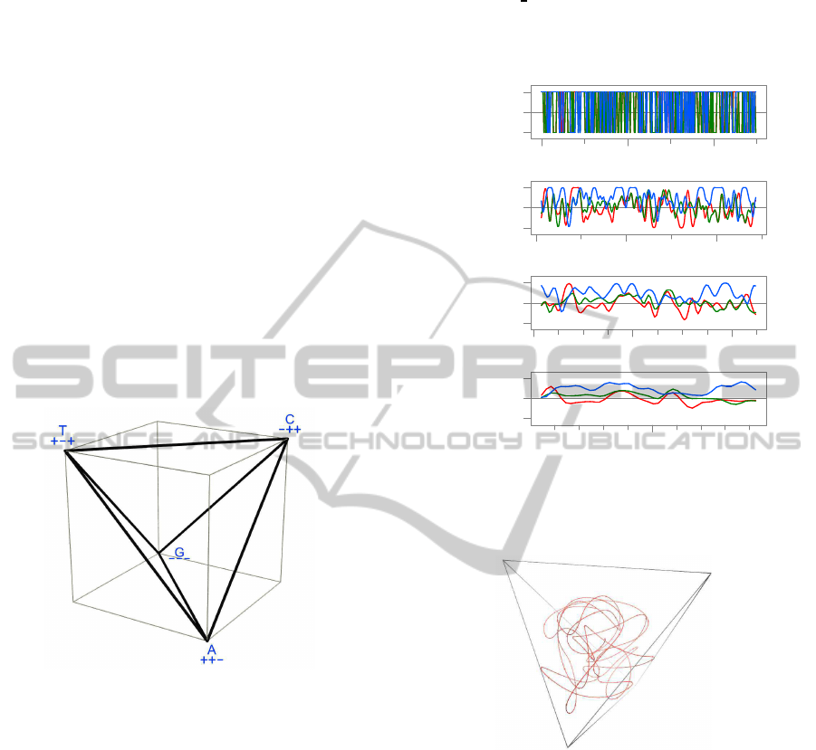
Figure 1: The tetrahedron T
3
whose corners encode the let-
ters of the DNA alphabet B.
3.1 Multiscale Analysis of DNA
In multi-scale signal analysis, a given discrete numer-
ical sequence X is transformed into a hierarchy of dis-
crete signals x
(0)
,..x
(m)
; where x
(0)
is the original se-
quence X, and each subsequent signal x
(k)
with k ≥ 1
is a downsampled version of the previous one x
(k−1)
,
with some step δ
(k)
≥ 1 (usually 2). With the encod-
ing described in section 3, multiscale analysis can be
applied to DNA sequences as well, by treating each
channel as a numeric discrete signal. See figure 2.
3.2 The Space-curve Representation
Each level x
(k)
of the multi-scale hierarchy of a DNA
sequence is a sequence of points x
(k)
[0],..x
(k)
[n −1]
in three-dimensional space. These points can be in-
terpolated with a cubic spline for any real argument t
in the range [0
n−1], to yield a smooth curve x
(k)
(t)
in three-dimensional space. This curve can be plotted
with arbitrary 3D rendering methods or viewed with
interactive 3D visualization tools. See figure 3.
x
(0)
0 100 200
-1.00
+0.00
+1.00
x
(1)
0 100 200
-1.00
+0.00
+1.00
x
(2)
0 100 200
-1.00
+0.00
+1.00
x
(3)
100
-1.00
+0.00
+1.00
Figure 2: Multiscale versions of a DNA sequence with 250
nucleotides, encoded as corners of T
3
, filtered and down-
sampled as described in section 4.2 and 4.3. The three chan-
nels are plotted in red, green, and blue, respecively.
Figure 3: Three-dimensional plot of a DNA segment from a
Drosophila sp. genome, originally with 250 nucleotides,
filtered by the w
(1)
filter of table 1, with no downsam-
pling, and then with the w
(2)
filter, downsampled with step
δ
(2)
= 2. The beads along the curve are the actual datums;
the connecting lines were reconstructed by cubic interpo-
lation. The entire curve was magnified by the scale factor
s = 1.440 relative to the origin (the center of the tetrahe-
dron) for clarity.
For k = 0, the curve intersects itself at a tetrahe-
dron vertex at every integer t, and therefore is quite
uninformative; but for k ≥ 1 self-intersections are
rare, and the general shape of the curve conveys useful
information, as we shall see. At successive stages, the
curve becomes necessarily simpler, losing the smaller
details (and being trimmed at each end) while retain-
ing the larger ones. See figure 4.
IVAPP2015-InternationalConferenceonInformationVisualizationTheoryandApplications
220

x
(1)
, s = 1.000 x
(2)
, s = 1.200 x
(3)
, s = 1.440 x
(4)
, s = 1.728
Figure 4: Three-dimensional plots of a DNA segment from a Drosophila sp. genome, originally with 500 nucleotides, filtered
and downsampled at various scales by the filter kernels of table 1. Each curve was magnified by the indicated scale factor s,
for clarity.
4 FILTERING AND
DOWNSAMPLING
4.1 Aliasing
As proved in signal theory, before downsampling a
discrete numeric signal x
(k−1)
to obtain x
(k)
, we must
make sure that x
(k−1)
contains no Fourier components
whose frequencies are at or above the Nyquist limit
(one cycle every 2δ
(k)
samples of x
(k−1)
). Otherwise,
the downsampling will turn those high-frequency
components into low-frequency ones, which will
be impossible to separate from the genuine low-
frequency components of x
(k)
. (This phenomenon is
known as frequency aliasing in signal theory.) Worse,
the downsampled sequence will vary drastically if the
sequence x
(k−1)
gets shifted by one position.
For example, consider the two DNA sequences
X
(0)
= (A, T, A,G,T,C,G, C, C,A)
Y
(1)
= (T, A, G,T,C,G,C, C, A,C)
(2)
Note that the sequence Y is basically X shifted 1 base
to the left. If we downsampled both sequences by
taking only the letters with even indices, we would get
X
(1)
= (A, A,T,G,C) and y
(1)
= (T, G,C,C). Now Y
(1)
appears to be x
(1)
shifted 2 bases to the left, which
would imply a shift of 4 bases at scale 0.
If the downsampled sequence is obtained by
averaging adjacent samples, namely if x
(k+1)
[i] =
(x
(k)
[2i] + x
(k)
[2i + 1])/2, the aliasing problem is
somewhat reduced, but still present. For example,
consider the two numeric sequences
x
(0)
= (0, 2,2,0,0,2, 2,0,0,2, 2, 0)
y
(1)
= (2, 2,0,0,2,2, 0,0,2,2, 0, 0)
(3)
The sequences obtained by averaging pairs of consec-
utive samples and downsampling with step 2 would
be x
(1)
= (1,1,1,1, 1, 1) and y
(1)
= (2,0,2,0, 2, 0).
4.2 Convolution Filtering
In order to avoid aliasing, we apply a smoothing con-
volution filter to each sequence x
(k−1)
before down-
sampling it to x
(k)
. The filtering from scale k −1 to
scale k is defined by a kernel radius L
(k)
and a ta-
ble w
(k)
of kernel weights w
(k)
[r] where r, defined
for r ∈ {−L
(k)
..+L
(k)
}. The downsampling is de-
fined by the sampling step δ
(k)
and a sampling offset
S
(k)
≥ L
(k)
. Namely,
x
(k)
[ j] =
∑
r
w
(k)
[r]x
(k−1)
[δ
k
j + S
(k)
−r]
∑
r
w
(k)
[r]
(4)
where the index r ranges from −L
(k)
to +L
(k)
.
Formula 4 is to be applied for all indices j such
that all indices in the right-and side are valid. There-
fore the length of the resulting sequence will be
n
(k)
=
j
(n
(k−1)
−(S
(k)
+ L
(k)
+ 1))/δ
(k)
k
+ 1; unless
n
(k−1)
< S
(k)
+ L
(k)
+ 1, in which case x
(k)
is empty
(n
(k)
= 0) by definition. The offset S
(k)
should prefer-
ably be chosen so that the new sequence is as long as
possible and approximately centered in the original.
4.3 Filtering Kernels and Steps
In the examples given in this paper, we use δ
(1)
= 1
(no downsampling) after the first filtering and δ
(k)
= 2
for subsequent stages k ≥2. The filter kernel we use is
w
(k)
[r] = W
(k)
[r]/D
(k)
, where W
(k)
and D
(k)
are given
in table 1. The power spectra of these two kernels are
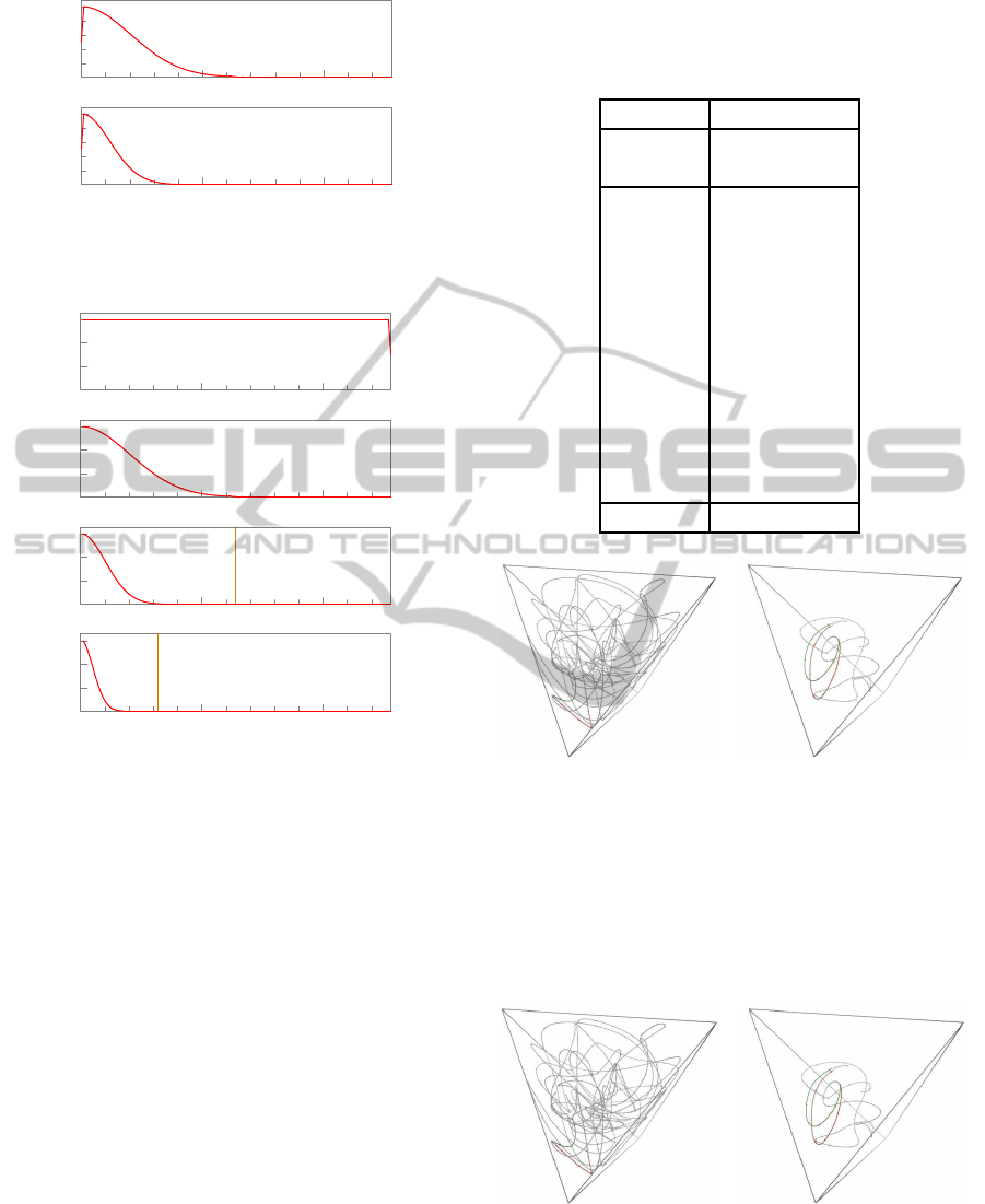
shown in figure 5.
These filtering kernels were chosen so that all signals
x
(k)
with k ≥1 have about the same degree of smooth-
ing. See figure 6. We define the degree of smoothing
U
(k)
recursively by U
(0)
= 0, and U
(k)
= (U
(k−1)
+
V
(k)
)/(δ
(k)
)
2
for all k ≥ 1; where V
(k)
is the variance
of the filtering kernel w
(k)
, interpreted as a probability
distribution on the indices {−L
(k)
..+L
(k)
}.
GeometricEncoding,Filtering,andVisualizationofGenomicSequences
221

50
100
+1.00
50
100
+1.00
Figure 5: Power spectra of the filtering kernels w
(k)
of ta-
ble 1, for the initial step k = 1 (top) and subsequent steps
k ≥ 2 (bottom).
50
100
+2.00
+4.00
+6.00
50
100
+2.00
+4.00
+6.00
50
100
+2.00
+4.00
+6.00
50
100
+2.00
+4.00
+6.00
Figure 6: Idealized power spectrum of an unfiltered peri-
odic random binary signal with a 256-sample period (top)
and its spectra after 1, 2, and 3 filtering steps. The vertical
line shows the maximum frequency that is preserved with-
out aliasing by the combined downsamplings from level 0
to the indicated level.
The quantity U
(k)
is an estimate of the variance of the
impulse response function of the linear process that
transforms the unfiltered sequence x
(0)
into x
(k)
. In
particular, the definition U
(0)
= 0 is consistent with
the fact that the original unfiltered sequence x
(0)
is not
smooth at all. With our choices of kernels and steps,
this recurrence gives U
(k)
= 2.00 for all k ≥ 1. We
take this to mean that all scales are smoothed to the
same degree, and equally safe from aliasing artifacts.
5 ROBUSTNESS
If one uses proper filtering before subsampling, the
resulting curve x
(k)
is robust under mutations of the
original sequence by replacement, insertions or dele-
tions of short nucleotide sequences. This claim is il-
lustrated in figures 7 and 8.
Table 1: Elements of the filtering kernels used in the ex-
amples. The last line V
(k)
is the variance of the kernel
w
(k)
, viewed as a probability distribution on the indices with
mean 0.
k = 1 k ≥ 2
L
(k)
6 10
D
(k)
35440 61364
W
(k)
[0] 9992 9992
W
(k)
[±1] 7786 9193
W
(k)
[±2] 3680 7161
W
(k)
[±3] 1055 4722
W
(k)
[±4] 183 2636
W
(k)
[±5] 19 1245
W
(k)
[±6] 1 498
W
(k)
[±7] 169
W
(k)
[±8] 48
W
(k)
[±9] 12
W
(k)
[±10] 2
V
(k)
2.00 6.00
x
(1)
, y
(1)
, s = 1.000 x
(3)
, y
(3)
, s = 1.440
Figure 7: Effect of a single-nucleotide substitution on the
filtered space curves of the same 250-nucleotide DNA se-
quence of figure 4, at scales k = 1 (left) and k = 3 (right).
The red curve x
(k)
(t) is derived from the original sequence,
the green curve y
(k)
(t) is derived from the mutated one. For
clarity, the curves were magnified by the indicated factor
s, and the parts where the two curves coincide were made
transparent.
x
(1)
, y
(1)
, s = 1.000 x
(3)
, y
(3)
, s = 1.440
Figure 8: Effect of a single-nucleotide insertion on the fil-
tered space curves of the same 250-nucleotide DNA se-
quence of figure 4, at scales k = 1 (left) and k = 3 (right),
with the same conventions as in figure 7.
IVAPP2015-InternationalConferenceonInformationVisualizationTheoryandApplications
222

In figure 8, note that the final segment of the modified
sequence y
(0)
has its datums shifted by one position
relative to the original sequence x
(0)
. That becomes
a shift by 1 position in y
(1)
, and by 0.25 positions in
y
(3)
. Nevertheless, as can be seen in the figure, the
interpolated curves still coincide, even in that part.
6 COMPARISON WITH OTHER
ENCODINGS
We claim that our three-channel encoding is better
suited for multi-scale analysis than other alternatives
that have been considered.
6.1 Why Not a Single-channel
Encoding?
An obvious alternative is to encode each letter by
a single distinct number — say, map A,T,C,G to
0,1,2,3 respectively. However, with this encoding
certain sequences consisting of very distinct bases
would map to the same averaged code when fil-
tered — a coincidence that has no biological justifi-
cation. For example, if X = (AGAGAG ...) and Y =
(TCTCTC ...) we would have x = (0, 3, 0,3,0,3, . . .)
and y = (1,2,1,2,1,2, . . .), which would produce ap-
proximately the same sequence (1.5, 1.5,...) when
filtered with a moderately wide kernel.
6.2 Why Not a Two-channel Encoding?
Another problem of this encoding is that the strength
of the Fourier spectrum of a pattern depends on which
nucleotides it uses. For example, the sinusoidal com-
ponents with period 2 in the sequences X and Y
above have amplitudes 3.0 and 1.0, respectively, even
though the patterns are basically the same (an alterna-
tion of two letters).
The same problems will inevitably occur if we
were to map each base to a two-component vector
or a complex number, as proposed by E. A. Cheever
et al. (Cheever et al., 1989) and used by L. Pessoa
et al. (Pessˆoa et al., 2004). In these works, each
base is represented by a complex number: A, T, C,
and G are mapped to +1, −1, +i, and − i, respec-
tively, where i =
√
−1 is the imaginary unit. For ex-
ample, with X = (ATATAT ...) and Y = (GCGCGC ...)
we would have x = (+1,−1, +1,−1,+1,−1,...) and
y = (+i,−i, +i,−i,+i,−i,...), and both would be-
come very close to (0, 0,...) when filtered with a
moderately wide kernel.
6.3 Why Not a Four-channel Encoding?
Another obvious alternative would be to use a four-
channel encoding where each letter is mapped to a
cardinal vector of R
4
; that is, where coordinate j of
x[i] is 1 if and only if X[i] is the j-th letter of the al-
lowed alphabet. Namely,
A → (1,0,0,0)
T → (0,1,0,0)
C → (0,0,1,0)
G → (0,0,0,1)
However, note that the sum of all four coordinates
will be always 1, not only for the individual codes
but also for for any average of codes. Thus the four-
channel codes actually lie on a three-dimensionalsub-
space of R
3
, meaning that the encoding is redundant.
Indeed, the four-channel codes of the DNA letters
are the corners of a regular three-dimensional tetra-
hedron T
4
in R
4
; and any weighted average of those
codes is a point of T
4
. Indeed there is a simple one-
to-one mapping from a point x
′
= (x
′
0
,x
′
1
,x
′
2
) of R
3
to
a point x
′′
= (x
′′
A
,x
′′
T
,x
′′
C
,x
′′
G
) of R
4
that maps T
3
to T
4
.
Namely,
x
′′
A
= ( + x
′
0
+ x
′
1
−x
′
2
+ 1)/4
x
′′
T
= ( + x
′
0
−x
′
1
+ x
′
2
+ 1)/4
x
′′
C
= ( −x
′
0
+ x
′
1
+ x
′
2
+ 1)/4
x
′′
G
= ( −x
′
0
−x
′
1
−x
′
2
+ 1)/4
(5)
Note that x
′′
A
+ x
′′
T
+ x
′′
C
+ x
′′
G
is always 1. It can be ver-
ified that the following projection of R
4
to R
3
is a
one-to-one mapping of T
4
to T
3
that is the inverse of
the above mapping:
x
′
0
= + x
′′
A
+ x
′′
T
−x
′′
C
−x
′′
G
x
′
1
= + x
′′
A
−x
′′
T
+ x
′′
C
−x
′′
G
x
′
2
= −x
′′
A
+ x
′′
T
+ x
′′
C
−x
′′
G
(6)
Therefore, we conclude that the 4-channel encoding
above contains exactly the same information as our
proposed 3-channel encoding.
7 CONCLUSIONS
We described a three-channel encoding of DNA se-
quences that is adequate for multi-scale analysis –
specifically, for filtering and anti-aliased resampling
– and allows visualization of the results as smooth
curves in three-dimensional space.
We foundthat the tetrahedral encodingof genomic
sequences described in this paper is convenient for vi-
sualization of genomic sequences of moderate length
(a few hundred nucleotides), especially after filtering
and subsampling. We also found that, with correct
GeometricEncoding,Filtering,andVisualizationofGenomicSequences
223

filtering, the three-dimensional shape of the subsam-
pled sequence is fairly insensitive to simple mutations
or insertions of short nucleotide sequences.
REFERENCES
Anastassiou, D. (2002). Digital signal processing
of biomolecular sequences. Technical Report
CU/EE/TR2000-20-042, Department of Electrical En-
gineering, Columbia University.
Cheever, E. A., Searls, D. B., Karunaratne, W., and Over-
ton, G. C. (1989). Using signal processing techniques
for DNA sequence comparison. Proceedings of 15th
Bioengineering Conference, pages 173–174.
Cristea, P. (2002). Conversion of nucleotides sequences into
genomic signals. Journal of Cellular and Molecular
Medicine, 6(2):279–303.
Futschik, A., Hotz, T., Munk, A., and Sieling, H. (2014).
Multiscale DNA partitioning: Statistical evidence for
segments. Bioinformatics, page btu180.
Knijnenburg, T. A., Ramsey, S. A., Berman, B. P., Kennedy,
K. A., Smit, A. F. A., Wessels, L. F. A., Laird, P. W.,
Aderem, A., and Shmulevich, I. (2014). Multiscale
representation of genomic signals. Nature Methods.
Machado, J. A. T., Costa, A. C., and Quelhas, M. D.
(2011). Wavelet analysis of human DNA. Genomics,
98(3):155–163.
Pessˆoa, L., Leit˜ao, H. C. G., and Stolfi, J. (2004). Mutual in-
formation content of homologous DNA sequences. In
Proc. 2004 Workshop on Bioinformatics (WOB), num-
ber 6016 in Lecture Notes on Informatics, pages 57–
64.
Ravichandran, L., Papandreou-Suppappola, A., Spanias,
A., Lacroix, Z., and Legendre, C. (2011). Waveform
mapping and time-frequency processing of DNA and
protein sequences. IEEE Transactions on Signal Pro-
cessing, 59(9):4210–4224.
Vincken, K. L., Koster, A. S. E., and Viergever, M. A.
(1997). Probabilistic multiscale image segmentation.
IEEE Transactions on Pattern Analysis and Machine
Intelligence, 19(2):109–120.
IVAPP2015-InternationalConferenceonInformationVisualizationTheoryandApplications
224