Sales Forecasting Models in the Fresh Food Supply Chain

Gabriella Dellino

, Teresa Laudadio

, Renato Mari

, Nicola Mastronardi

and Carlo Meloni

1,2

Istituto per le Applicazioni del Calcolo ”M. Picone”, Consiglio Nazionale delle Ricerche, Bari, Italy

Dipartimento di Ingegneria Elettrica e dell’Informazione, Politecnico di Bari, Bari, Italy

Keywords:

Fresh food supply chain, Forecasting, ARIMA, ARIMAX, Transfer function.

Abstract:

We address the problem of supply chain management for a set of fresh and highly perishable products. Our

activity mainly concerns forecasting sales. The study involves 19 retailers (small and medium size stores)

and a set of 156 different fresh products. The available data is made of three year sales for each store from

2011 to 2013. The forecasting activity started from a pre-processing analysis to identify seasonality, cycle

and trend components, and data ﬁltering to remove noise. Moreover, we performed a statistical analysis to

estimate the impact of prices and promotions on sales and customers’ behaviour. The ﬁltered data is used

as input for a forecasting algorithm which is designed to be interactive for the user. The latter is asked to

specify ID store, items, training set and planning horizon, and the algorithm provides sales forecasting. We

used ARIMA, ARIMAX and transfer function models in which the value of parameters ranges in predeﬁned

intervals. The best setting of these parameters is chosen via a two-step analysis, the ﬁrst based on well-known

indicators of information entropy and parsimony, and the second based on standard statistical indicators. The

exogenous components of the forecasting models take the impact of prices into account. Quality and accuracy

of forecasting are evaluated and compared on a set of real data and some examples are reported.

1 INTRODUCTION

Supply chain optimization is one of the most chal-

lenging tasks in operation management due to the

presence of multiple critical issues and multiple deci-

sion makers involved. Inventory management, order

planning, scheduling and vehicle routing are among

the most studied problems in the logistic ﬁeld (Ja-

cobs and Chase, 2014) in order to reduce supply chain

and transportation costs, and to increase service level,

quality and sustainability.

The efﬁciency and effectiveness of quantitative

methods for optimizing a supply chain strictly depend

on the quality of available data. It is often assumed

that customer demand is available and/or it is deter-

ministic, while in real scenarios this assumption does

not hold and future sales are often a missing data. For

this reason, sales forecasting represents the ﬁrst cru-

cial step for such an optimization process and may

affect the capacity to design a realistic supply chain

model.

In the market of fresh and highly perishable food

sales forecasting plays an even more important role

since the shelf life of products is very limited and re-

liable forecasts are fundamental to reduce and man-

age inefﬁciencies such as stock out and outdating. In

this paper, we address the problem of sales forecast-

ing for a set of fresh and highly perishable products

analyzing real data coming from a set of medium and

small size retailers operating in Apulia region, Italy.

Data was pre-processed to remove noise and identify

basic components, such as trends, cycles and season-

ality. The pre-processed data was used to design three

different forecasting models taking into account the

effect of exogenous variables, such as prices, on sales

behaviour. The ﬁrst two models are based on ARIMA

multiplicative models (Box et al., 2008), while the

third is a more sophisticated transfer function model

(Makridakis et al., 2008). The three models were

identiﬁed and estimated by varying parameters in pre-

deﬁned intervals. The best parameter setting was

selected based on a statistical analysis and a set of

performance indicators. A ﬁnal step consists in em-

bedding these forecasting models within an algorith-

mic framework designed to be interactive for the user

and operating as a decision support system for supply

chain management.

The rest of the paper is organized as follows. In

Section 2 we describe the structure and characteristics

of our data set, and the adopted pre-processing tech-

niques. In Section 3 we provide theoretical insight

on multiplicative ARIMA models and present the ﬁrst

419

Dellino G., Laudadio T., Mari R., Mastronardi N. and Meloni C..

Sales Forecasting Models in the Fresh Food Supply Chain.

DOI: 10.5220/0005293204190426

In Proceedings of the International Conference on Operations Research and Enterprise Systems (ICORES-2015), pages 419-426

ISBN: 978-989-758-075-8

 2015 SCITEPRESS (Science and Technology Publications, Lda.)

forecasting model. In Section 4 we describe the sta-

tistical analysis and performance indicators used for

model selection. In Section 5 we describe the second

and the third forecasting models designed to take the

impact of exogenous variables into account. Finally,

in Section 6 we provide some examples, while con-

clusions are given in Section 7.

2 DATA DESCRIPTION

The data set used for designing and setting the fore-

casting models comes from a real fresh food supply

chain. The available data is made of three year sales,

from 2011 to 2013, for a set of 19 retailers of small

and medium size operating in Apulia region in Italy.

We selected a subset of 156 fresh products belonging

to the category of best sellers for which the available

sales were characterized by large and reliable num-

bers.

Concerning the model implementation, we di-

vided the given data set into two different time sets: a

training set and a test set. The training set represents

the set of observations used to estimate the forecast-

ing model and its parameters. Once the model has

been estimated, we run it taking the test set as input

and deriving forecasts on this set. Then, we compare

forecasted sales with real sales over the test set. Thus,

the test set provides the forecasting horizon.

The training set is used to perform the so-called

in-sample analysis, while the test set is used to com-

pare forecast to observed data, assess the efﬁcacy of

the forecasting model and perform the so-called out-

of-sample analysis. Both analyses rely on statistical

indicators which are described in the following sec-

tion.

2.1 Pre-processing

Data collected for model estimation needed to be pre-

processed for a two-fold reason: identify trends, cy-

cles and seasonality, and remove noise. A seasonality

of 7 days was observed, that is typical of food sold

on large scale distribution in which customers tend to

have well deﬁned cyclical behaviour.

Once the training set is deﬁned, sales are normal-

ized as follows. Let y

be the quantity of product P

sold in store V at time t. Then, the corresponding nor-

malized quantity z

− µ

, (1)

where µ and σ are the sample mean, respectively, and

the standard deviation of time series y

over the train-

ing set.

Besides we attempted to ﬁlter data using more so-

phisticated approaches based on independent compo-

nent analysis (Hyv

arinen and Oja, 2001), that are typ-

ically used in signal and image processing. However

it did not provide remarkable quality improvements

for our data set. The reader is referred to (Najarian

and Splinter, 2005) for a detailed description of ad-

vanced data processing techniques.

3 ARIMA MODELS

A time series can be considered as the realization of

a stochastic process that is observed sequentially over

time. Thus, once a time series of data is collected,

it is possible to identify a mathematical model to de-

scribe the stochastic process. The study of theoretical

properties of the deﬁned model allows to perform a

statistical analysis of the time series and forecast fu-

ture values for the series.

A well known class of mathematical models for

time series forecasting is represented by the Autore-

gressive Integrated Moving Average (ARIMA) mod-

els (Box et al., 2008). ARIMA models are widely

used in statistics, econometrics and engineering for

several reasons: (i) they are considered as one of the

best performing models in terms of forecasting, (ii)

they are used as benchmark for more sophisticated

models, (iii) they are easily implementable and have

high ﬂexibility due to their multiplicative structure.

Let z

be the realization of a stochastic process at

time t, that is an observation of time series at time

t, and let a

be a random variable with normal distri-

bution, having zero mean and variance equal to σ

Thus, the random variable a

represents the realiza-

tion at time t of a white noise process. An ARIMA

model with seasonality is deﬁned as follows:

(B)Φ

)∇

∇

= θ

(B)Θ

, (2)

where B is the backward shift operator which is de-

ﬁned by Bz

= z

t−1

and

(B) = 1 − φ

B − φ

.. . − φ

, (3)

) = 1 − Φ

− Φ

.. . − Φ

, (4)

(B) = 1 − θ

B − θ

.. . − θ

, (5)

) = 1 − Θ

− Θ

.. . − Θ

, (6)

∇

= (1 − B)

, (7)

∇

= (1 − B

)

. (8)

The parameter p deﬁnes the order of the autoregres-

sive non-seasonal component AR, q deﬁnes the order

of the moving average non-seasonal component MA,

ICORES2015-InternationalConferenceonOperationsResearchandEnterpriseSystems

420

and the parameter d represents the order of non sea-

sonal integration necessary to obtain a stationary time

series. The parameters p, q and d are commonly used

for referring to non-seasonal models in a concise way.

For more complex models, in which similar pattern

at regular time intervals can be observed, it is more

realistic to take seasonality under consideration. A

data set comprised of food sales on large-scale stores

is typically affected by a weekly seasonality, which

reﬂects the customers’ habit to buy foods especially

in the weekend. The seasonal component is deﬁned

by the parameters P, D and Q, where P deﬁnes the

order of the autoregressive non-seasonal component

SAR, Q deﬁnes the order of the moving average non-

seasonal component SMA, and D is the order of sea-

sonal differences. Finally, s deﬁnes the series’ sea-

sonality. A seasonal ARIMA model is synthetically

described as ARIMA(p,d,q) × (P,D,Q)

. The most

critical disadvantage of classical ARIMA models with

seasonality is that the effect of exogenous variables on

data is not taken into account. In the following sec-

tions we show how to cope with this issue, and to this

end we present two alternative forecasting models.

According to (Box et al., 2008), given a data set,

the best forecasting model can be identiﬁed according

to the following framework:

• model identiﬁcation,

• model estimation,

• diagnostic check.

In the literature the model identiﬁcation is imple-

mented through either an incremental approach or an

exhaustive one. In the ﬁrst approach the value of

the parameters deﬁning the ARIMA model are iter-

atively incremented and statistical signiﬁcance tests

are performed for halting. The simplest way to im-

plement this approach is to deﬁne the parameter d as

follows: it starts setting d = 0 and testing the time se-

ries stationarity by statistical tests; based on the result

of the latter, either d is incremented or the process is

halted. For a complete application of the incremental

approach see, for instance, (Andrews et al., 2013). On

the contrary, in the exhaustive approach each param-

eter ranges in predeﬁned intervals; see for instance

oglund and

Ostermark, 1991). The main advantage

of this approach is that a larger set of combinations,

i.e., forecasting models, are compared and the result-

ing model is more accurate. However, the computa-

tional effort required may be larger, since for every

ARIMA model a set of statistical tests and analyses

have to be performed. In the proposed forecasting

models, we implemented the incremental approach

for parameters p, d, q, P, D and Q and we set sea-

sonality s = 7.

For each tuple (p,d,q) × (P,D, Q)

the maximum

likelihood principle is adopted for model parame-

ters’ estimation. Finally the diagnostic check of the

forecasting model is implemented by means of two

kinds of performance indicators, in-sample and out-

of-sample, that are used to determine the best model.

In the following section we analyze the diagnostic

check phase in more detail and provide a complete

description of the performance indicators used within

our forecasting models.

4 PERFORMANCE INDICATORS

In this section we describe a set of statistical indica-

tors used to assess the forecasting quality of the mod-

els. These indicators can be divided into two groups,

in-sample and out-of-sample indicators, according to

the set of data used for computing them. For the sake

of clearness, we describe the latter separately as their

meaning, as well as their use, is different within the

proposed forecasting models.

4.1 In-sample Indicators

This subset includes indicators that are computed on

the training set as deﬁned in Section 2. These are

mostly used as lack of ﬁt measures, based on the in-

formation entropy and parsimony of models. Thus,

in-sample analysis has the objective to measure the

matching between real data and simulated data ob-

tained by the mathematical model under analysis.

We computed two different indicators: the Ljiung-

Box test and the Hannan-Quinn Information Criterion

(HQC) (Box et al., 2008), (Burnham and Anderson,

2002). The Ljiung-Box test is a a portmanteau test in

which the null hypothesis is that the ﬁrst m autocorre-

lations of the residuals r

are zero, i.e. they are like a

white process noise. The statistical test applied in this

study is

Q(m) = n(n + 2)

∑

h=1

n − h

, (9)

which follows a χ

(m − K) distribution with m − K

degrees of freedom, where K is the number of param-

eters estimated within the model and n is the num-

ber of observations in the test set. The Hannan-Quinn

Information Criterion (HQC) is a well known crite-

rion used to quantify the entropy of the information

and the information lost in the ﬁtting process. Under

the assumption that the residuals are independent and

identically distributed,

HQC = n log(SSR/n) + 2K loglog(n), (10)

SalesForecastingModelsintheFreshFoodSupplyChain

421

holds, where SSR is the Sum of Squared Residu-

als. The HQC represents a compromise between the

Akaike Information Criterion (AIC) and the Bayesian

Information Criterion (BIC) and tends to penalize

lack of parsimony, that is a high value of the param-

eter K. The interested reader is referred to (Burn-

ham and Anderson, 2002) for a detailed description of

these in-sample indicators and others. For the sake of

implementation of our forecasting models, the latter

indicators are used as follows: it is performed a non

domination analysis with respect to variance, residu-

als and HQC for all the models obtained by chang-

ing the tuple (p, d, q) × (P,D,Q)

. The dominated

models, as well as models not satisfying the Ljung-

Box test, are excluded by the following diagnostic

check, while the remaining models undergo the out-

of-sample analysis.

4.2 Out-of-sample Indicators

The out-of-sample indicators are well known statisti-

cal indicators for quality and accuracy of forecasting

and they are computed on the test set. This implies

that they are used to compare forecast data and real

data within the test set and allow to make a quantita-

tive comparison among different models in terms of

quality of forecast. The ﬁrst group of indicators in-

cludes absolute measures: they are scale dependent

and for this reason can only be used when different

indicators are computed on the same data set, but can

not be used to compare the behaviour of a forecast-

ing model on different data sets. Let us deﬁne f

the forecast of quantity of product P sold in store V

at time t and with test set {1,...,n}. We compute the

following indicators:

• Root Mean Squared Error (RMSE):

∑

t=1

− f

)

• Mean Absolute Error (MAE):

∑

t=1

− f

• Maximum Absolute Error (MaxAE):

max

t=1,...,n

− f

The second set of indicators is comprised of relative

measures that are not scale dependent. On the one

hand, it is possible to compare the same model on

different scale data sets, but on the other hand these

measures are not deﬁned for time t in which z

= 0.

Thus, it is preferable not to use them with either miss-

ing data or data too close to zero. We computed the

following indicators:

• Mean Absolute Percentage Error (MAPE):

100 ·

∑

t=1



− f



• Maximum Absolute Percentage Error (MaxAPE):

max

t=1,...,n



− f



• Coefﬁcient of determination R

1 −

∑

t=1

− f

)

∑

t=1

− µ)

where µ is the average value of z

over the test set.

There are many works in the literature concerning

with statistical indicators. The reader is referred

to (Makridakis et al., 2008), (Makridakis and Hi-

bon, 2000) and (Armstrong, 2001) for a complete

overview. Among non-dominated models with re-

spect to in-sample indicators, we selected the model

with minimum MAE concluding the diagnostic check

and, hence, the model selection. Alternative (possi-

bly multi-objective) criteria could be chosen; how-

ever, our choice for the MAE was based on experts’

opinion, as retailers are mostly interested in minimiz-

ing the absolute deviation from actual sales.

5 EXOGENOUS VARIABLES

The main drawback of classical ARIMA models is

the lack of information about the impact of exoge-

nous variables on the time series. In many cases it

may be more realistic to take the impact of external

phenomena into account. In the case study under in-

vestigation, it is easy to understand that sales of fresh

goods are highly inﬂuenced by prices and the impact

of the latter on the forecasting process should be con-

sidered. In the literature several approaches can be

found to make forecasting more robust and reliable

including the effect of exogenous variables, in partic-

ular of prices. To this end, we designed two more

sophisticated forecasting models: the ﬁrst is a gen-

eralization of the classical ARIMA model, while the

second follows a slightly different approach based on

transfer function theory. Both models are ﬂexible and

can be used with any kind of exogenous variable.

5.1 ARIMAX Models

ARIMA model with exogenous variables, also re-

ferred to as ARIMAX, can be deﬁned as follows:

(B)Φ

)∇

∇

= θ

(B)Θ

+ βx

, (11)

where x

is the vector of exogenous variables and β

is the vector of regression coefﬁcients. The latter has

ICORES2015-InternationalConferenceonOperationsResearchandEnterpriseSystems

422

to be estimated and its initial value is set equal to the

canonical correlation between z

(series of sales) and

(series of prices). According to (Makridakis et al.,

2008), the deﬁnition of β as regression coefﬁcient is

not properly correct. Indeed, the ARIMAX can be

restated as

∇

(B)Θ

)

(B)Φ

)

(B)Φ

)

, (12)

which clearly points out that the relationship between

and x

is not linear. The authors propose a slight

modiﬁcation of the previous ARIMAX model, that is

a regression model with ARIMA error in which there

is an explicit linear relation between z

and x

plus

an error component that is described by an ARIMA

model. More formally

= βx

+ n

, (13)

where n

is the error vector described by an ARIMA

model. (Makridakis et al., 2008) showed that the fore-

cast quality of a regression model with ARIMA er-

ror (13) is almost comparable with the quality of an

ARIMAX model (11) and the difference between the

two models is not remarkable. Therefore, we imple-

mented an ARIMAX forecast model as it is more sim-

ilar to classical ARIMA model and we believe that a

comparison between ARIMA and ARIMAX models

is more meaningful.

The general framework used to select the best

ARIMAX model reproduces the one described above,

and it is based on the same three phases of model

identiﬁcation, model estimation and diagnostic check

(see Section 3).

5.2 Transfer Function Models

The third forecasting model we developed is based on

the assumption that the relation between time series

and exogenous variables can be modeled by a trans-

fer function (to be estimated) plus an error vector de-

scribed by an ARIMA model. More formally,

ω(B)B

δ(B)

+ n

, (14)

where the transfer function is deﬁned by s poles, r

zeros and a delay b, with

ω(B) = 1 − ω

B − ω

.. . − ω

, (15)

δ(B) = 1 − δ

B − δ

.. . − δ

, (16)

and the vector of errors n

is described by the follow-

ing ARIMA model

(B)Φ

)∇

∇

= θ

(B)Θ

. (17)

Unlike the previous two models, in this third one ad-

ditional parameters have to be estimated, namely pa-

rameters s, r and b. The exhaustive approach previ-

ously described for model identiﬁcation is performed,

thus parameters s, r range in predeﬁned intervals,

while parameter b is estimated according to the max-

imum likelihood principle. In order to perform an in-

sample analysis and choose the best value of unknown

parameters, for each pair (s, r) the simulated time se-

ries ˆz

is deﬁned as

ˆz

ω(B)B

δ(B)

, (18)

The original time series z

is compared to ˆz

and the

following goodness of ﬁt measure F is computed

F = 100 ·

1 − kz − ˆzk

kz − µk

, (19)

where µ is the average value of z

over the training set.

The pair (s,r) providing the best ﬁtting F is selected

and the error vector is computed as n

= z

− ˆz

. The

algorithmic approach used to deﬁne the best ARIMA

model for n

is the same described in the previous sec-

tion.

Therefore, a transfer function model will be de-

scribed by a tuple (p, d, q) × (P, D,Q)

× (s,r,b),

whose values will be identiﬁed as discussed so far.

6 EXAMPLES

In this section we compare the three forecasting mod-

els previously described, testing them on a set of real

sales data. All forecasting models are implemented

in Matlab. The out-of-sample indicators are used to

assess the quality of the forecast provided. Note that,

in our implementation, the user is required to specify

store and item, retrieved by a database, along with the

time intervals deﬁning training set and test set, and

what kind of exogenous variables has to be accounted

for.

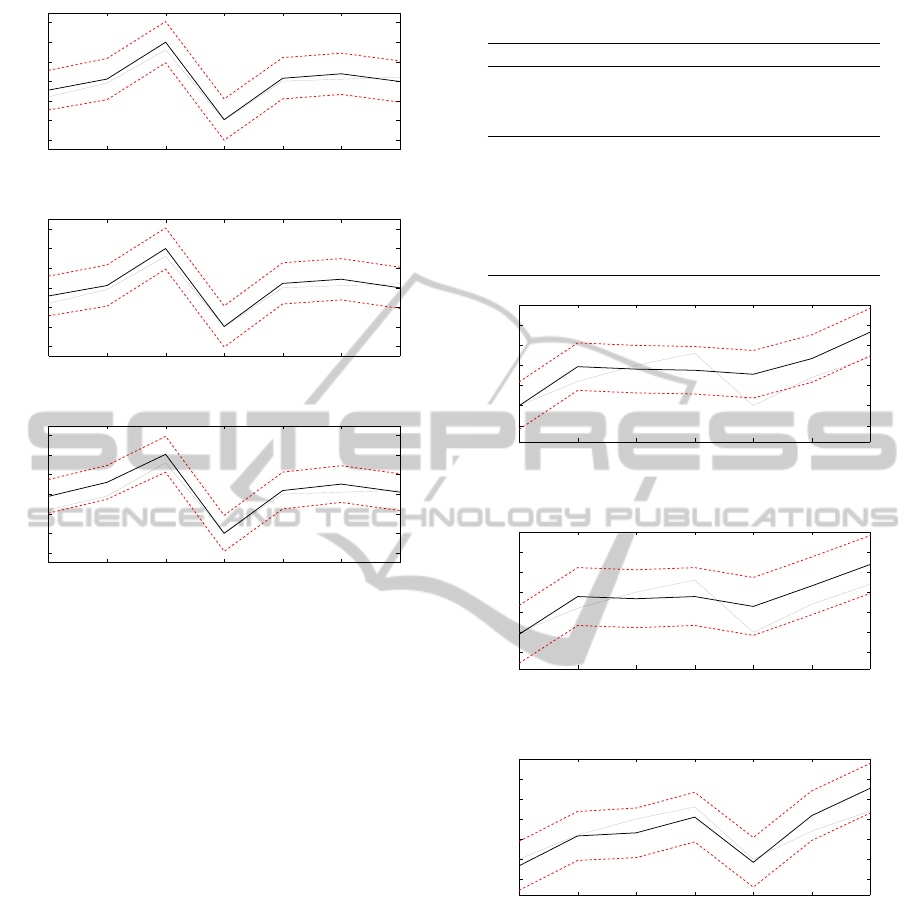
The ﬁrst example refers to a common fresh item,

1 liter of milk, considering a training set of 90 days

and a test set of 7 days. Recall that the test set also

represents the forecasting horizon. In Figures 1, 2

and 3 observed data are depicted with a grey line,

forecasts with a black line and the red dashed lines

represent the 95% conﬁdence interval for the fore-

cast. ARIMA and ARIMAX models provide similar

forecasts, while those based on the transfer function

model deviate more from the actual sales, especially

over the ﬁrst half of the forecasting horizon.

SalesForecastingModelsintheFreshFoodSupplyChain

423

1075 1076 1077 1078 1079 1080 1081

−10

days

sales

Figure 1: Sales forecast based on ARIMA for milk.

1075 1076 1077 1078 1079 1080 1081

−10

days

sales

Figure 2: Sales forecast based on ARIMAX for milk.

1075 1076 1077 1078 1079 1080 1081

−10

days

sales

Figure 3: Sales forecast based on transfer function model

for milk.

Table 1 compares the performance of the three

forecasting models, the bold values denoting the best

value among the three.

The analysis based on out-of-sample indicators

conﬁrms that ARIMA and ARIMAX models have a

quite similar performance, even though the ARIMA

model seems to be the best performing model accord-

ing to the adopted statistical indicators. Notice that,

for the ARIMA model, a MAPE of 13.48% corre-

sponds to a MAE of 2.31: this means that, on average,

we observe a forecast error of approximately 2 liters

of milk w.r.t. observed sales, with a worst case of less

than 4 liters (MaxAE = 3.94). The transfer function

model does not perform very well and the difference

is remarkable, especially for the MaxAPE.

In the second example we computed the forecast

for another very common fresh product, 250 grams of

mozzarella cheese, on the same training set of 90 days

and test set of 7 days. Comparison plots are reported

in Figures 4, 5 and 6 while Table 2 shows results for

the statistical indicators we computed.

In this case the transfer function model is the

best performing while the forecast quality of ARIMA

and ARIMAX models is almost the same, as already

emerged from the corresponding ﬁgures. Again we

notice that a MAPE of 31.92%, which might suggest

Table 1: Out-of-sample analysis for milk.

ARIMA ARIMAX TR FUN

(p, d,q) (0,0, 1) (0,0, 1) (2,0, 0)

(P,D, Q)

(1,1, 1)

(s,r,b) - - (2,2, 0)

RMSE 2.57 2.79 4.44

MAE 2.31 2.51 3.62

MaxAE 3.94 4.05 7.06

MAPE 13.48% 14.93% 23.34%

MaxAPE 28.44% 31.24% 57.32%

93.50% 92.32% 80.64%

840 841 842 843 844 845 846

−5

days

sales

Figure 4: Sales forecast based on ARIMA for mozzarella

cheese.

840 841 842 843 844 845 846

−5

days

sales

Figure 5: Sales forecast based on ARIMAX for mozzarella

cheese.

840 841 842 843 844 845 846

−5

days

sales

Figure 6: Sales forecast based on transfer function model

for mozzarella cheese.

a relatively inaccurate model, corresponds instead to

less than 3 units of products (MAE = 2.59).

Finally, the third example considers 200 grams of

salmon. Plots are showed in Figures 7, 8 and 9, while

the out-of-sample analysis is reported in Table 3.

The transfer function model seems to be the best

model in terms of RMSE, MAE, MaxAE and R

, even

though the ARIMAX model performs slightly better

as far as MAPE and MaxAPE are concerned. How-

ever, it is worth noting that, for the ARIMAX model,

smaller percentage errors (in terms of both MAPE

and MaxAPE) still implies higher absolute errors (in

ICORES2015-InternationalConferenceonOperationsResearchandEnterpriseSystems

424

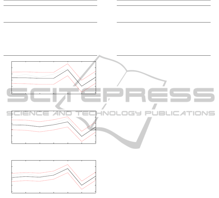
Table 2: Out-of-sample analysis for mozzarella cheese.

ARIMA ARIMAX TR FUN

(p, d,q) (1,1, 2) (0,0, 0) (2,0, 0)

(P,D, Q)

(1,1, 1)

(1,0, 0)

(1,1, 0)

(s,r,b) - - (3,2, 0)

RMSE 4.69 4.05 3.13

MAE 3.94 3.58 2.59

MaxAE 7.78 6.45 5.65

MAPE 44.45% 40.46% 31.92%

MaxAPE 66.79% 65.26% 54.90%

8.82% 32.17% 59.52%

610 611 612 613 614 615 616

−20

days

sales

Figure 7: Sales forecast of ARIMA for salmon.

610 611 612 613 614 615 616

−20

days

sales

Figure 8: Sales forecast of ARIMAX for salmon.

610 611 612 613 614 615 616

−20

days

sales

Figure 9: Sales forecast of transfer function model for

salmon.

terms of MAE and MaxAE). Instead, the opposite oc-

curs for the transfer function model, which suggests

that a single performance indicator may not sufﬁce to

identify the best forecasting model. Nevertheless, in

this case, the ARIMA model is clearly outperformed

by the other two forecasting models.

Summing up these examples, it is evident that

there is no forecasting model clearly outperforming

the others, but the performance strictly depends on the

data set. ARIMAX models either dominate ARIMA

ones or they provide almost comparable results, while

the transfer function appears the most ﬂexible model,

as it can be easily adapted to cope with different ex-

ogenous variables. By an overall analysis, the trans-

Table 3: Out-of-sample analysis for salmon.

ARIMA ARIMAX TR FUN

(p, d,q) (1,0, 0) (1,0, 0) (2,0, 2)

(P,D, Q)

(0,1, 1)

(1,0, 1)

(s,r,b) - - (3,2, 0)

RMSE 6.94 5.34 5.21

MAE 4.96 4.21 4.08

MaxAE 13.74 11.51 10.15

MAPE 15.50% 11.05% 13.06%

MaxAPE 35.23% 20.56% 26.70%

80.24% 88.31% 88.87%

fer function model seems to be the model to prefer in

terms of forecasting accuracy and potentiality.

We now compare our forecasted sales with fore-

casts currently estimated by the management, based

on sales observed in the previous week. Comput-

ing out-of-sample indicators for management’s fore-

casted data for the selected sample products, we no-

tice that adopting rigorous forecasting methods usu-

ally pays off in terms of forecast accuracy. In fact, all

the three proposed forecasting models clearly domi-

nate the actual forecasting system, for both milk and

mozzarella cheese. More speciﬁcally, the actual man-

agement forecasting not only shows the worst MAE

(MAE

milk

= 4.14, MAE

mozzarella

= 5.57), but also

performs worse than the proposed models over all the

selected out-of-sample indicators. As for salmon, we

recall that the transfer function model and the ARI-

MAX model showed non-dominated performance in-

dicators; the management forecasts (MAE

salmon

4.57) appear worse than those provided by the afore-

mentioned models.

The ﬁnal aim of this research is to design a deci-

sion support system in which the proposed forecast-

ing models are embedded. In fact, this forecasting

tool will be the basis for an order planning system.

Once real sales data becomes available, it is possible

to compare forecasted and real data, assess the quality

of forecasting and then either keep the current model

or estimate new model parameters. Then, based on

forecasted sales, management takes decisions on the

quantity to order for each item, and the correspond-

ing frequency. A detailed description of the decision

support system goes beyond the scope of this paper.

As a preliminary investigation, we depict poten-

tial implications of adopting our forecasting models

on the order policy, comparing the effects with those

related to the actual management. For instance, we

consider the case of mozzarella cheese, whose shelf

life is 18 days and minimum order quantity is of one

unit. We assume to place a single order at the begin-

ning of the planning horizon, aiming at covering all

the week demand. Sales in the previous week were

SalesForecastingModelsintheFreshFoodSupplyChain

425

67 units; thus, the actual policy would suggest to or-

der the same quantity. Instead, our best forecasting

model predicts sales for 49 units, which determines

the order quantity. The real sales are 48 units; there-

fore, our order proposal would imply a stock reduc-

tion of 18 units.

7 CONCLUSIONS

In this paper we described three different forecasting

models and compared their performances on a real

data set comprised of three year sales for fresh and

highly perishable foods. Due to the short shelf life of

products, accurate sales forecasting is a crucial issue

for supply chain management and optimization.

We developed an ARIMA model and two more

complex models, an ARIMAX model and a transfer

function model, in order to include the effect of ex-

ogenous variables, such as prices, and obtain more

realistic and reliable forecasts. All the models were

selected according to a standard algorithmic frame-

work comprised of three phases: model identiﬁcation,

model estimation and diagnostic check. We made use

of classical statistical indicators to select the best fore-

casting model. We reported some examples to com-

pare the forecasting quality of the three models. Our

preliminary results show that it is not possible to iden-

tify a model that is clearly the best performing one,

since the forecasting quality strictly depends on the

data set. Nevertheless, the transfer function model

seems to be the most ﬂexible and reliable one. Be-

sides, this model deﬁnitely dominates the actual man-

agement forecasting system: this result further sup-

ports the usefulness of adopting rigorous forecasting

methods, rather than relying on management experi-

ence, which might leave speciﬁc hidden trends unno-

ticed. Additional beneﬁts are related to order policy

implications, as more accurate forecasts enable to re-

duce potential stock-outs and, even more important

for fresh products, outdating.

Future research may develop along two paths: on

the one side, it may focus on using more sophisticated

tools for model selection, improving forecast accu-

racy by means of non scale-dependent indicators and

considering the impact of other exogenous variables,

e.g. promotion and festivities. On the other side, it

may address the development of an automatic order

planning system, precisely aiming at managing stock-

out and outdating reduction.

ACKNOWLEDGEMENTS

This work was supported by the E-CEDI project,

funded by P.O. Puglia, Asse I FESR 2007-2013 Linea

1.2 – Azione 1.2.4.

REFERENCES

Andrews, B. H., Dean, M. D., Swain, R., and Cole, C.

(2013). Building arima and arimax models for pre-

dicting long-term disability beneﬁt application rates

in the public/private sectors. Technical report, Society

of Actuaries and University of Southern Maine.

Armstrong, J. S. (2001). Principles of Forecasting: A Hand-

book for Researchers and Practitioners. Springer.

Box, G. E. P., Jenkins, G. M., and Reinsel, G. C. (2008).

Time Series Analysis: Forecasting and Control. Wiley,

4th edition.

Burnham, K. P. and Anderson, D. R. (2002). Model

Selection and Multimodel Inference: A Practical

Information-Theoretic Approach. Springer.

oglund, R. and

Ostermark, R. (1991). Automatic arima

modelling by the cartesian search algorithm. Journal

of Forecasting, 10(5):465–476.

Hyv

arinen, A. and Oja, E. (2001). Independent Component

Analysis. Wiley.

Jacobs, F. and Chase, R. (2014). Operations and Supply

Chain Management. McGrawHill/Irwin, 14th edition.

Makridakis, S. and Hibon, M. (2000). The m3-competition:

results, conclusions and implications. International

Journal of Forecasting, 16(4):451–476.

Makridakis, S., Wheelwright, S. C., and Hyndman, R. J.

(2008). Forecasting Methods and Applications. Wiley

India Pvt. Limited, 3rd edition.

Najarian, K. and Splinter, R. (2005). Biomedical Signal and

Image Processing. Taylor & Francis.

ICORES2015-InternationalConferenceonOperationsResearchandEnterpriseSystems

426