Resilient Propagation for Multivariate Wind Power Prediction
Jannes Stubbemann, Nils Andre Treiber and Oliver Kramer
Department of Computer Science, University of Oldenburg, 26111 Oldenburg, Germany
Keywords:
Neural Networks, Resilient Propagation, Wind Power Prediction.
Abstract:
Wind power prediction based on statistical learning has the potential to outperform classical physical weather
prediction models. Neural networks have been successfully applied to wind prediction in the past. In this
paper, we apply neural networks to the spatio-temporal prediction model we proposed in the past. We con-
centrate on a comparison between classical backpropagation and the more advanced resilient propagation
(RPROP) variants. The analysis is based on time series data from the NREL western wind data set. The
experimental results show that RPROP+ and iRPROP+ significantly outperform the classical backpropagation
variants.
1 INTRODUCTION
While physical models for wind power predictions
have advantages in long-term range, statistical meth-
ods perform well for short-term predictions (Lei et al.,
2009). With this motivation, we have built a spatio-
temporal prediction model and employed linear, k-
nearest neighbor and support vector regression tech-
niques in the past (Kramer et al., 2013; Treiber et al.,
2013). In this paper, we experimentally compare re-
silient propagation (RPROP) variants to enhance the
methodological repertoire of regression methods for
wind power prediction based on the spatio-temporal
model.
The paper is structured as follows. In Section 2,
we introduce the wind power prediction problem as
regression problem and present related work. RPROP
and its variants are shortly sketched in Section 3. The
experimental comparison is presented in Section 4.
Results are summarized and discussed in Section 5.
2 WIND POWER PREDICTION
The power grid is moving from a stable supply of
comparatively few centralized power plants to a het-
erogenous grid with thousands of entities. Their
power is fluctuating and depending on wind and sun.
For a stable integration of renewables into the grid,
a precise prediction is important. Since a couple of
years data-driven models have shown to deliver com-
petitive results in wind power prediction.
2.1 Wind Prediction as Regression
Problem
We treat the wind power prediction problem as regres-
sion problem. Given a training set of pattern-label ob-
servations {(x
1
, y
1
), . . . , (x
N
, y
N
)} ⊂ R
d
, we seek for
a regression model f : R
d
→ R that learns reason-
able predictions for power values of a target turbine
given unknown patterns x
0
. We define the patterns as
wind power features x
i
∈ R
d
of a target turbine and its
neighbors at time t (and the past) and the labels as tar-
get power values y
i
at time t + λ. Such wind power
features x
i
= (x
i,1
, . . . , x
i,d
)
T
can consist of present
and past measurements, i.e., p
j
(t), . . . , p
j
(t − µ) of
µ ∈ N
+
time steps of turbine j ∈ N from the set
N of employed turbines (target and its neighbors) or
wind power changes p
j
(t −1) − p
j
(t), . . . , p
j
(t −µ) −
p
j
(t − µ + 1). In the experimental evaluation of this
work, we construct each pattern with µ = 2 past mea-
surements and only consider absolute values (and no
differences).
2.2 Related Work
Neural networks have been applied to data-based
wind prediction in the past. For example, Mohandes
et al. compared an autoregressive model with a clas-
sical backpropagation network for wind speed predic-
tion and demonstrated the superior accuracy of the
neural network model (Mohamed A. Mohandes and
Halawani, 1998). In a similar line of research, Cata-
lao et al. trained a three-layered feedforward network
333
Stubbemann J., Andre Treiber N. and Kramer O..
Resilient Propagation for Multivariate Wind Power Prediction.
DOI: 10.5220/0005284403330337
In Proceedings of the International Conference on Pattern Recognition Applications and Methods (ICPRAM-2015), pages 333-337
ISBN: 978-989-758-077-2
Copyright
c
 2015 SCITEPRESS (Science and Technology Publications, Lda.)

with the Levenberg-Marquardt algorithm for short-
term wind power forecasting, which outperformed the
persistence model
1
and ARIMA approaches (Catalao
et al., 2009). Han et al. focused on an ensemble
method of neural networks for wind power prediction
(Han et al., 2011).
In our preliminary work, we proposed the spatio-
temporal approach for support vector regression
in (Kramer et al., 2013) that has been introduced in
the previous section. In (Treiber et al., 2013), we con-
centrated on the aggregation of features with nearest
neighbors and support vector regression on the level
of a wind park. Recently, we proposed an ensemble
approach based on statistical learning methods (Hein-
ermann and Kramer, 2014). An evolutionary method
for feature selection has been proposed by (Treiber
and Kramer, 2014).
3 RESILIENT PROPAGATION
RPROP has been introduced as variant of backprop-
agation to allow faster learning and avoiding oscillat-
ing around local optima.
3.1 Backpropagation
The backpropagation learning algorithm for training
of feedforward networks has originally been intro-
duced by Rumelhart et al. (Rumelhart et al., 1986).
It is based on fitting the network output o
net
to the tar-
get values y
i
given pattern x
i
. This can be written as
error function
2
E
net
:
E
net
=
1
2
N
∑
i=0
((y
i
− o
net
(x
i
)
2
) (1)
In backpropagation, the weights of the network w
i j
are adapted via gradient descent
w
(t+1)
i j
= w
(t)
i j
+ ∆w
(t)
i j
(2)
with
∆w
(t)
i j
= −ρ ·
∂E
∂w
i j
(t)
(3)
and learning rate ρ. As a variant, backpropagation
with momentum (BPMom) considers the last weight
update in the current update
∆w
(t)
i j
= −ρ ·
∂E
∂w
i j
(t)
+ α · ∆w
(t−1)
i j
(4)
to reduce oscillations around local optima.
1
The naive persistence model assumes that the wind will
not change within time horizon λ.
2
The definition corresponds to the mean squared error
(MSE) of the prediction.
3.2 RPROP
RPROP has been introduced as extension of classi-
cal backpropagation by Riedmiller and Braun (Ried-
miller and Braun, 1992). The idea of RPROP is to
replace the constant learning rate ρ by adaptive step
sizes ∆
i j
that are controlled during learning for each
weight w
i j
. The step sizes ∆
i j
are updated as follows
∆
(t)
i j
=







∆
(t−1)
i j
· η
+
if
∂E
∂w
i j
(t)
·
∂E
∂w
i j
(t−1)
> 0
∆
(t−1)
i j
· η
−
if
∂E
∂w
i j
(t)
·
∂E
∂w
i j
(t−1)
< 0
∆
(t−1)
i j
else
(5)
with parameters 0 < η
−
< 1 < η
+
, which specify the
step size adaptation magnitude, if the sign of the gra-
dient
∂E
∂w
i j
(t−1)
changes. The weights are updated with
∆w
(t)
i j
= −sign(
∂E
∂w
i j
(t)
) · ∆
(t)
i j
(6)
Two RPROP variants that include backtracking are in-
troduced in the following.
1 for each w
i j
do
2 if
∂E
∂w
i j
(t−1)
·
∂E
∂w
i j
(t)
> 0 then
3 ∆
(t)
i j
:= min(∆
(t−1)
i j
· η
+
, ∆
max
)
4 ∆w
(t)
i j
:= −sign(
∂E
∂w
i j
) · ∆
(t)
i j
5 w
(t+1)
i j
:= w
(t)
i j
+ ∆w
(t)
i j
6 elseif
∂E
∂w
i j
(t−1)
·
∂E
∂w
i j
(t)
< 0 then
7 ∆
(t)
i j
:= max(∆
(t−1)
i j
· η
−
, ∆
min
)
8 w
(t+1)
i j
:= w
(t)
i j
− ∆w
(t)
i j
9
∂E
∂w
i j
(t)
:= 0
10 elseif
∂E
∂w
i j
(t−1)
·
∂E
∂w
i j
(t)
= 0 then
11 ∆w
(t)
i j
:= −sign(
∂E
∂w
i j
) · ∆
(t)
i j
12 w
(t+1)
i j
:= w
(t)
i j
+ ∆w
(t)
i j
Algorithm 1: Pseudocode of RPROP+, oriented
to Igel and H
¨
usken (Igel and H
¨
usken, 2003).
The weight update is reverted in case the sign
of the partial derivative has changed.
3.3 RPROP+
RPROP+ is an extension of RPROP and has been
introduced by Igel and H
¨
usken (Igel and H
¨
usken,
2003). The idea of RPROP+ is to revert the weight
update step in case the sign of the partial derivative
ICPRAM2015-InternationalConferenceonPatternRecognitionApplicationsandMethods
334

has changed. Algorithm 1 shows the pseudocode of
RPROP+. If the sign of the partial derivative has
not changed in the last iteration, the step size ∆
i j
of
weight w
i j
increases. The step size is limited by the
maximum value ∆
max
. If the sign of the gradient has
changed in the last iteration, step size ∆
(t)
i j
is decreased
(again limited by the minimum value ∆
min
) and the
last weight update is reverted. Last, the current gra-
dient is reset to 0 to enforce the last condition (Line
12), which conducts a weight update with the new (re-
duced) step size.
Figure 1 illustrates with working principle of
RPROP+. An increase of the step size in case the sign
of the partial derivative has not changed is reasonable
5 Backpropagation-Varianten
der Gewichte berechnet. Durch die Multiplikation der Schrittweite in 5.5 mit dem um-
gekehrten Vorzeichen ≠sign(
ˆE
ˆw
ij
) des Gradienten werden die Gewichte w
ij
immer in
Richtung des Gefälles der Fehlerfunktion verändert.
Christian Igel und Michael Hüsken haben 2003 in [8] vier unterschiedliche Varianten
aus dem Algorithmus von Riedmiller und Braun herausgestellt. Zwei dieser Varianten,
„Resilien Propagation with weight-backtracking“ (RPROP+) und „improved Resilient
Propagation with Backtracking“ (iRPROP+) werden in den nächsten zwei Abschnit-
ten vorgestellt. Sie unterscheiden sich lediglich in der Hinsicht, ob der letzte Schritt
rückgängig gemacht wird, wenn sich das Vorzeichen des Gradienten verändert hat.
w
(t)
ij
w
(t+4)
ij
w
ij
E(w
ij
)
Abbildung 5.1: Die Schrittweite wird bei RPROP jedes Mal erhöht, wenn sich das Vorzeichen
des Gradienten zum vorherigen Schritt nicht geändert hat. Ändert es sich, wird
der letzte Schritt rückgängig gemacht und die Schrittweite für den nächsten
Schritt verkleinert. So wird verhindert, dass die Gewichte um das Minimum
oszillieren.
5.3.1 RPROP+
Die erste von Igel und Hüsken beschriebene Variante von RPROP ist „RPROP with
backtracking“ (RPROP+). Hierbei wird der letzte Schritt rückgängig gemacht, wenn sich
das Vorzeichen des letzten und das des aktuellen Gradienten voneinander unterscheiden.
In Abb. 5.2 ist der Ablauf des RPROP+-Algorithmus zu sehen.
30
Figure 1: Illustration of gradient descent with RPROP+.
to accelerate the walk into the direction of the opti-
mum (left two solid arrows). In case the optimum
is missed and the sign of the partial derivates have
changed (dotted arrow), the following gradient de-
scent step is performed from the previous position
with a decreased step size (w
t+4
).
3.4 iRPROP+
A further method we test is the improved resilient
propagation with backtracking (iRPROP+) (Igel and
H
¨
usken, 2003), which is an extension of RPROP+.
The difference to RPROP+ is that the weight update
is only reverted, if it led to an increased error, i.e., if
E
(t)
> E
(t−1)
. In pseudocode 1, Line 9 must be re-
placed by
IF E
(t)
> E
(t−1)
THEN w
(t+1)
i j
:= w
(t)
i j
− ∆w
(t)
i j
The variants are experimentally compared in the next
section.
4 EXPERIMENTAL ANALYSIS
In this section, we compare standard backpropaga-
tion, backpropagation with momentum, RPROP+,
and iRPROP+ experimentally. For this sake, the
four methods are run for 2000 iterations on test data
sets in turbines from Casper, Las Vegas, Reno, and
Tehachapi for a prediction horizon of λ = 3 steps (30
minutes). We use each 5th pattern of the wind time
series data of year 2004. The resulting data set con-
sists of 10512 patterns, of which 85% are used for
training and 15% are randomly drawn for the valida-
tion set. Each training process is repeated three times.
The topologies of the neural networks depend on the
number of employed neighboring turbines, which de-
termine the dimensionality of patterns x
i
:
• Casper: 33 input neurons (10 neighboring tur-
bines, 1 target turbine, 3 time steps), 34 hidden
neurons
• Cheyenne: 33 input neurons (10 neighboring tur-
bines, 1 target turbine, 3 time steps), 34 hidden
neurons
• Las Vegas: 30 input neurons (9 neighboring tur-
bines, 1 target turbine, 3 time steps), 31 hidden
neurons
• Reno: 30 input neurons (9 neighboring turbines,
1 target turbine, 3 time steps), 31 hidden neurons
• Tehachapi: 21 input neurons (6 neighboring tur-
bines, 1 target turbine, 3 time steps), 22 hidden
neurons
For the classical backpropagation variants, the fol-
lowing parameters are chosen: ρ = 3 · 10
−7
and
α = 1 · 10
−8
for BPMom. For RPROP, the fol-
lowing parameters are chosen: ∆
min
= 1 · 10
−6
,
∆
max
= 50, η
−
= 0.5, and η
+
= 1.2. Table 1 shows
the experimental results. The figures show the vali-
dation error in terms of MSE. RPROP+ and iRPROP
clearly outperform the two classical backpropagation
variants.
In the following, we analyze and compare the
learning curves of BP and RPROP. Figure 2 shows
the validation error development in terms of MSE in
the course of backpropagation and iRPROP+ train-
ing for the Tehachapi data sets. The plots show that
RPROP+ achieves a significantly faster training error
reduction than backpropagation. A closer look at the
learning curves (in terms of validation error) offers
Figure 3. Each three runs of backpropagation show a
smooth approximately linear development. iRPROP+
based training reduces the errors faster, but also suf-
fers from slight deteriorations during the learning pro-
cess. However, the situation changes at later stages of
ResilientPropagationforMultivariateWindPowerPrediction
335

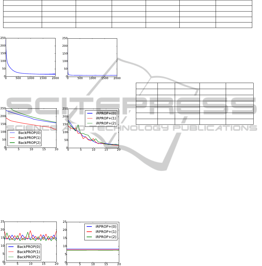
Table 1: Comparison of standard backpropagation (BackPROP), backpropagation with momentum (BackPROPMom),
RPROP+ and iRPROP+ in terms of validation error (MSE).
Algorithm Casper Cheyenne Las Vegas Reno Tehachapi ∅
BackPROP 19.51(8.73%) 19.32(15.17%) 14.82(9.64%) 16.9(9.34%) 17.66(13.36%) 17.64(11.25%)
BackPROPMom 19.45(8.3%) 20.62(13.41%) 14.32(6.2%) 16.35(3.45%) 18.02(9.33%) 17.75(8.14%)
RPROP+ 10.57(3.87%) 8.37(4.12%) 10.83(3.97%) 12.32(3.32%) 7.62(3.04%) 9.94(3.66%)
iRPROP+ 10.76(5.08%) 8.56(3.83%) 10.92(3.52%) 12.47(3.11%) 7.81(3.9%) 10.1(3.89%)
(a) BP (b) iRPROP+
Figure 2: Learning curve for training of (a) backpropagation
and (b) iRPROP+ training on Tehachapi for 2000 iterations.
(a) BP (b) iRPROP+
Figure 3: Learning curve for training of (a) backpropaga-
tion and (b) iRPROP+ training on Tehachapi for the first 20
training iterations.
learning, see Figure 4, which shows the last 20 itera-
tions. Here, the backpropagation learning curves fluc-
tuate, while the iRPROP+ training curves converge
smoothly to constant values.
(a) BP (b) iRPROP+
Figure 4: Learning curve for training of (a) backpropaga-
tion and (b) iRPROP+ training on Tehachapi for the last 20
training iterations.
The analyzed methods reach the optimum faster
than in 2000 iterations. Table 2 analyzes how fast
the optimum is reached, i.e. the number of training
iterations until the optimal validation error has been
reached. The experiments show that RPROP+ and iR-
PROP+ reach their optima faster than the backpropa-
gation variants. On Casper, Las Vegas and Reno, they
need far less than 1000 iterations for an optimal train-
ing. iRPROP+ is on average 37% faster than classic
BackPROP and 32% faster than BackPROPMom.
Table 2: Average number of iterations until minimum val-
idation error has been reached for all four neural networks
on five parks.
Park BP BPMom RPROP+ iRPROP+
Casper 1090 1025 936 919
Chey. 997 702 1316 803
L.V. 1339 1421 908 735
Reno 1999 1993 650 551
Teh. 1220 1015 1645 1190
∅ 1328 1231 1091 839
The results confirm that both RPROP variants out-
perform backpropagation. Further, iRPROP+ is up to
one third faster than RPROP+.
In the last part of the experimental analysis, we
show the results of RPROP in time series predic-
tion scenarios. The prediction results of iRPROP+
on a short exemplary interval are shown in the fol-
lowing. Figure 5(a) shows a comparison between the
predicted wind power of iRPROP+, the persistence
model PST, and the real measurements y. The fig-
ure shows that the curve of iRPROP+ is closer to the
curve of y. This observation is confirmed by the plot
of deviations, see Figure 5(b). The iRPROP+ devia-
tion from the real wind power is in most cases smaller
than the deviation than PST. Interestingly, ramp-up
events are over-estimated, i.e., they are predicted ear-
lier than they occur.
5 CONCLUSIONS
In this work, we applied neural networks to the
spatio-temporal time series regression approach for
the first time. The experimental analysis has shown
that the two RPROP variants RPROP+ and iRPROP+
have outperformed the standard backpropagation al-
gorithms. The conditional acceptance of gradient de-
scent steps turns out to be advantageous for learning
the short term wind power prediction. In the future,
we will extend the experimental results to get statisti-
cally significant results and enlarge the number of test
data sets.
ICPRAM2015-InternationalConferenceonPatternRecognitionApplicationsandMethods
336

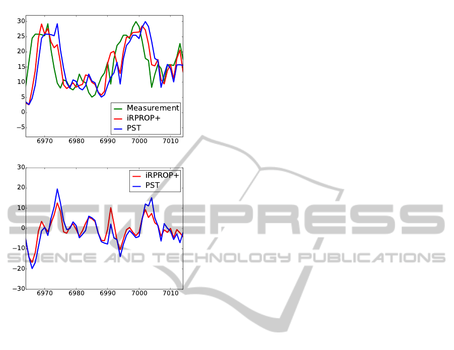
(a) prediction with iPROP+
(b) deviation from measurement
Figure 5: Prediction of wind power for short time interval
with iRPROP+ on Tehachapi (a) prediction and (b) devia-
tion from target values y
i
In further experiments, we observed that the
backpropagation variants outperform the persistence
model, nearest neighbor regression, and linear regres-
sion. We expect to improve the RPROP results with
an adaptation of the network architecture, e.g. with
GPROP (Castillo et al., 2000), which tunes the net-
work topology and initial parameters with genetic al-
gorithms. Further, we plan to apply deep learning to
the spatio-temporal prediction scenario.
ACKNOWLEDGEMENTS
We thank the National Renewable Energy Laboratory
(NREL) for the western wind data set.
REFERENCES
Castillo, P. A., Merelo, J. J., Prieto, A., Rivas, V., and
Romero, G. (2000). G-prop: Global optimization of
multilayer perceptrons using GAs. Neurocomputing,
35:149–163.
Catalao, J. P. S., Pousinho, H. M. I., and Mendes, V. M. F.
(2009). An artificial neural network approach for
short-term wind power forecasting in portugal. In In-
telligent System Applications to Power Systems, 2009.
ISAP ’09. 15th International Conference on, pages 1–
5.
Han, S., Liu, Y., and Yan, J. (2011). Neural network ensem-
ble method study for wind power prediction. In Power
and Energy Engineering Conference (APPEEC), 2011
Asia-Pacific, pages 1–4.
Heinermann, J. and Kramer, O. (2014). Precise wind power
prediction with SVM ensemble regression. In Artifi-
cial Neural Networks and Machine Learning - ICANN
2014 - 24th International Conference on Artificial
Neural Networks, Hamburg, Germany, September 15-
19, 2014. Proceedings, pages 797–804.
Igel, C. and H
¨
usken, M. (2003). Empirical evaluation of the
improved rprop learning algorithm. Neurocomputing,
50:105–123.
Kramer, O., Gieseke, F., and Satzger, B. (2013). Wind en-
ergy prediction and monitoring with neural computa-
tion. Neurocomputing, 109:84–93.
Lei, M., Shiyan, L., Chuanwen, J., Hongling, L., and Yan,
Z. (2009). A review on the forecasting of wind speed
and generated power. Renewable and Sustainable En-
ergy Reviews, 13(4):915 – 920.
Mohamed A. Mohandes, S. R. and Halawani, T. O. (1998).
A neural networks approach for wind speed predic-
tion. Renewable Energy, 13(3):345 – 354.
Riedmiller, M. and Braun, H. (1992). Rprop - a fast adaptive
learning algorithm. Proc. of ISCIS, VII.
Rumelhart, D., Hintont, G., and Williams, R. (1986). Learn-
ing representations by back-propagating errors. Na-
ture, 323:533–536.
Treiber, N. A., Heinermann, J., and Kramer, O. (2013). Ag-
gregation of features for wind energy prediction with
support vector regression and nearest neighbors. In
European Conference on Machine Learning, DARE
Workshop.
Treiber, N. A. and Kramer, O. (2014). Evolutionary turbine
selection for wind power predictions. In KI 2014: Ad-
vances in Artificial Intelligence - 37th Annual German
Conference on AI, Stuttgart, Germany, September 22-
26, 2014. Proceedings, pages 267–272.
ResilientPropagationforMultivariateWindPowerPrediction
337