Detection of Low-textured Objects
Christopher Bulla and Andreas Weissenburger
Institut f
¨
ur Nachrichtentechnik, RWTH Aachen University, Aachen, Germany
Keywords:
Object Detection, Local Features, SIFT.
Abstract:
In this paper, we present a descriptor architecture, SIFText, that combines texture, shape and color information
in one descriptor. The respective descriptor parts are weighted according to the underlying image content, thus
we are able to detect and locate low-textured objects in images without performance losses for textured objects.
We furthermore present a matching strategy beside the frequently used nearest neighbor matching that has
been especially designed for the proposed descriptor. Experiments on synthetically generated images show the
improvement of our descriptor in comparison to the standard SIFT descriptor. We show that we are able to
detect more features in non-textured regions, which facilitates an accurate detection of non-textured objects.
We further show that the performance of our descriptor is comparable to the performance of the SIFT descriptor
for textured objects.
1 INTRODUCTION
A problem often occurring in computer vision tasks is
the detection or recognition of identical objects within
different images. In recent years, invariant local fea-
tures (Lowe, D.G., 2004; Bay et al., 2006) have been
introduced to solve this problem. A local feature is a
n-dimensional vector, that contains a unique descrip-
tion of an image patch. An image typically contains
several local features and the entirety of all local im-
age features can be regarded as the description of the
image. If two or more images contain identical objects
a subset of their features will be identical or similar.
This could be used to detect common objects across
different images (Bulla and Hosten, 2013).
Many local feature approaches (e.g. SIFT, SURF)
are designed to detect meaningful image patches and
describe their gradient distribution. Therefore, they
could be well used to describe textured objects or im-
ages (cf. figure 1(a)). When they are used to describe
low-textured objects (cf. figure 1(b)) two problems oc-
cur: Firstly, low-textured objects only have high gradi-
ents at their border. Therefore most of the local image
patches are detected at the border and not on the object
itself. Secondly, when the patches at the border are de-
scribed, a large amount of the information covered by
the feature characterizes the background. Since low-
textured objects usually have a unique gradient-less
surface, the part of the feature that covers the object
doesn’t contribute much to the description.
In the literature several approaches have been in-
troduced to describe low-textured objects. The Bunch
Of Lines Descriptor (Tombari et al., 2013) for exam-
ple approximate the contour of an object by polygons
and describes this polygons. The Boundary Struc-
ture Segmentation approach (Toshev et al., 2012) uses
the chordiogram, a multidimensional histogram, to
describe a by superpixel segmented image and the
Distinct Multi-Colored Region Descriptors approach
(Naik and Murthy, 2007) describes the objects by re-
gions with different colors. All approaches are indeed
able to describe low-textured objects, but have in com-
mon that they lower the ability to describe textured
objects.
In this paper we present a combination of three de-
scriptors in order to describe low-textured, as well as
textured objects. We thereby combine texture, shape
and color information into a single descriptor and
weight each descriptor component based on the im-
age content. In textured regions e.g. we give a higher
weight to the texture descriptor, while in non-textured
regions the shape descriptor gets a higher weight. We
furthermore use a matching strategy apart the well
known nearest neighbor matching which allows an
accurate object localization.
The rest of the paper is organized as follows. In
chapter 2 we present our descriptor architecture. The
matching strategy will be presented in chapter 3. These
are evaluated in chapter 4. Finally conclusions will be
drawn in chapter 5.
265
Bulla C. and Weissenburger A..
Detection of Low-textured Objects.
DOI: 10.5220/0005269602650273
In Proceedings of the 10th International Conference on Computer Vision Theory and Applications (VISAPP-2015), pages 265-273
ISBN: 978-989-758-090-1
Copyright
c
 2015 SCITEPRESS (Science and Technology Publications, Lda.)

2 DESCRIPTOR
ARCHITECTURE
Our descriptor, SIFText has been designed to increase
the performance of SIFT in low-textured regions,
while maintaining its performance in textured regions.
We therefore combine texture, shape and color infor-
mation into a single descriptor and weight each de-
scriptor part by a locally calculated value, derived
from the texture of the image. As texture descriptor
we use SIFT, the shape will be described with ART
coefficients and the color descriptor is a combination
of Hue- and Opponent-Angle histograms. The sin-
gle descriptor parts as well as their weighting will be
described in the following subsections.
2.1 SIFT
Scale Invariant Feature Transform (SIFT) has been
published in 2004 by Lowe (Lowe, D.G., 2004) and
describes the content of an image patch by a histogram
of gradient orientations.
The selection of feature points is done in a scale
invariant way. In a first step the image I(x, y) is con-
volved with variable scale Gaussians G(x, y, σ ), and
the Difference-of-Gaussians (DoG) D(x, y, σ) is calcu-
lated:
D(x, y, σ) = I(x, y) ∗[G(x, y, kσ) −G(x, y, σ)] (1)
= L(x, y, kσ) −L(x, y, σ) .
Possible feature positions are given by the extrema
of these DoG images across all scales and image reso-
lutions. A refinement step selects the most distinctive
feature points and interpolates their exact position.
To make the descriptor invariant to object orienta-
tion, one or more dominant orientations are calculated
for each feature point. The dominant orientations are
given by the peaks of a weighted orientation histogram,
(a) Textured image and its
gradients
(b) Low-textured image and
its gradients
Figure 1: Gradients of a textured and a low-textured image.
which is formed from the gradient orientations Θ(x, y)
of sample points within a region around the point:
Θ(x, y) = tan
−1

L(x, y + 1) −L(x, y −1)
L(x + 1, y) −L(x −1, y)

. (2)
The weighting factors are given by the gradient magni-
tude m(x, y):
m(x, y) =
q
(L(x + 1, y) −L(x −1, y))
2
) + (3)
q
(L(x, y + 1) −L(x, y −1))
2
.
To build the descriptor the region around the feature is
divided into several sub-region and again, a weighted
histogram of gradient orientations is calculated for
each sub-region. The descriptor is given by the con-
catenation of all sub-histograms.
2.2 Shape
Low-textured objects can be well described by their
shape. We use Maximally Stable External Regions
(MSER) (Matas et al., 2004) to detect significant
shapes in an image and describe them with a set of
Angular Radial Transform (ART) (Bober, 2001) coef-
ficients.
Maximally Stable Extremal Regions are connected
regions that are characterized by an approximately
uniform intensity surrounded by a contrasting back-
ground. Furthermore, they are stable across a range
of thresholds on the intensity function. In order to
avoid segmentation errors on the edges of the MSER
regions (e.g. due to blurring artifacts in case of large
scale changes), we detect the MSER regions, similar
to SIFT, on multiple octaves (cf. (Forssen and Lowe,
D.G., 2007)). A morphological closing filter is applied
on the detected region, subsequent to the detection to
minimize noise within the region.
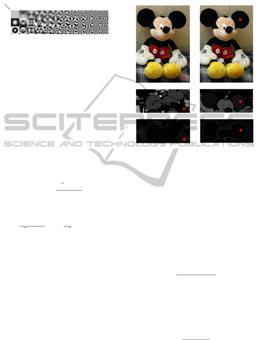
Figure 3 shows the detected MSER regions for one
image and visualizes the difference between a MSER
region and and a feature that has been detected on the
textured area of the image.
To calculate a descriptor from the maximal stable
regions we use ART, which describes the shape of a
region with the coefficients F
m,n
:
F
n,m
=
Z
2π
0
Z
1
0
V
∗
n,m
(ρ, Θ)I(ρ, Θ)ρ δρ δΘ (4)
In equation 4, I(ρ, Θ) is an image in polar coordinates
(e.g. a MSER region) and V
∗
n,m
a ART basis function:
V
n,m
(ρ, Θ) =
1
2π
e
jmΘ
R
n
(ρ) (5)
R
n
(ρ) =

1, if n = 0
2cos(πnρ), if n 6= 0
(6)
VISAPP2015-InternationalConferenceonComputerVisionTheoryandApplications
266

0 1 2 3 4 5 6
7
8 9 10 11 12
0
1
2
n
m
Figure 2: ART basis functions (real part).
Figure 2 depicts exemplarily the real parts of the fist
36 ART basis coefficients.
The coefficients are scale and translation invariant.
A rotation causes a shift in the coefficients phase. To
achieve rotation invariance we only use the coefficients
real part.
2.3 Color
The combination of SIFT and color has been exten-
sively studied in the literature (Van De Weijer and
Schmid, C., 2006). We used a combination of Hue-
and Opponent-Angle histograms in our descriptor ar-
chitecture. The Hue descriptor is suited for the descrip-
tion of high-saturated images, while the Opponent-
Angle descriptor is proper for the description of low-
saturated images.
Hue is the angle between the difference of RGB
color channels and can be computed as:
Hue = atan
√
3(G −B)
2R −G −B
!
. (7)
The Opponent-Angles are the partial derivatives in x-
and y- direction of the Opponent-Colors:
O
1
=
1
√
2(R −G)
, O
2
=
1
√
6
(R + G −2B) (8)
2.4 Descriptor Weighting and Fusion
In order to combine the individual descriptors, it is nec-
essary to normalize them. Therefore, each descriptor
will be normalized to unit length and the final descrip-
tor is a weighted combination of the three normalized
descriptors. The weighting factors steer the influence
of each individual descriptor to the total descriptor.
We choose the weighting factor for each feature point
adaptively, based on the image content. In the left part
of figure 3 a feature on a textured region is depicted.
Here, we have distinctive gradient information, but no
maximal stable region. Therefore the SIFT descriptor
for this feature point should have more influence on
the total descriptor than the shape descriptor. The op-
posite holds for the feature point in the right part of
figure 3.
Image
MSER regions
Gradient magnitude
Figure 3: Difference between MSER regions and gradient
based regions. Left: Keypoint in textured area with almost
no shape information. Right: MSER region with almost no
gradient information.
2.4.1 Weighting Factors for SIFT and SHAPE
The weighting factors for textured and non-textured
regions will be defined through the Gray Level Co-
occurrence Matrix (GLCM). The GLCM C
δ
i, j
is the
distribution of co-occurring intensity values ( i, j ) at a
given offset δ = (δ
x
, δ
y
) in an image of size (I
m
, I
n
):
C
δ
i, j
=
I
n
∑
p=1
I
m
∑
q=1

1, if i(p, q) = i ∧I(p + δ
x
, q + δ
y
) = j
0, else.
(9)
The weighting factor α can, with the number of gray
levels N
G
be computed as:
α =
∑
N
G
i=0
(C
1,1
i,i
)
2
∑
N
G
i=0
∑
N
G
j=0
(C
1,1
i, j
)
2
. (10)
For a homogeneous region, α will be equal to one,
while for a checkerboard pattern α will converge to
zero. The behaviour of alpha for some synthetically
generated texture pattern is depicted in figure 4. To
precisely steer the impact of α on the individual de-
scriptor parts, we mapp α to a sigmoid. As result of
this mapping we get the weighting factor a:
a =
1
1 + e
−bα−σ
0
. (11)
The parameter b in equation 11 could be used to create
either linear or threshold-like behavior of the sigmoid,
DetectionofLow-texturedObjects
267

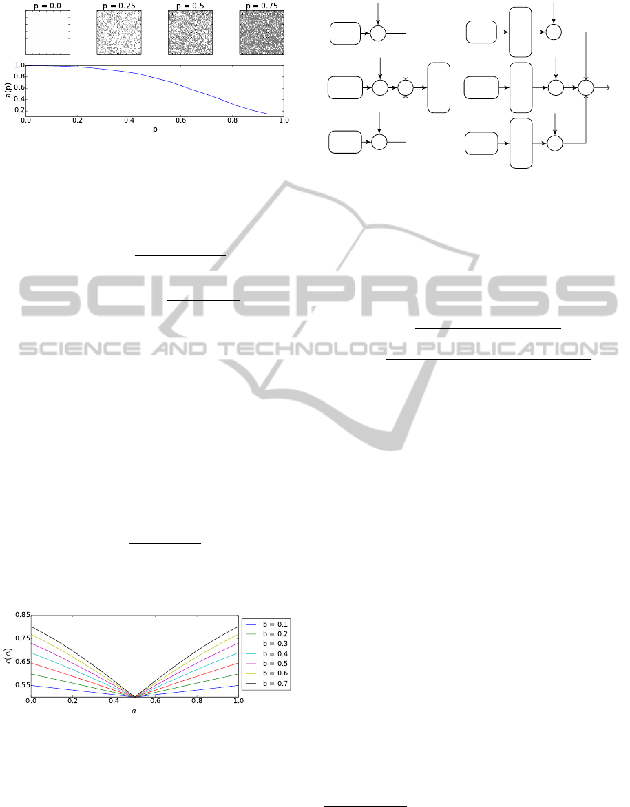
Figure 4: GLCM example.
while σ
0
could be used to prefer one descriptor part.
The normalized shape and SIFT descriptors f
0SHAPE
and f
0SIFT
are thus given by:
f
0SHAPE
= a
f
SHAPE
∑
N
SHAPE
j=0
|f
SHAPE
j
|
(12)
f
0SIFT
= (1 −a)
f
SIFT
∑
N
SIFT
j=0
|f
SIFT
j
|
, (13)
with N
SHAPE
, N
SIFT
denoting the number of elements
in the shape and texture descriptor
2.4.2 Weighting Factor for COLOR Descriptor
The color descriptor itself has, due to its construc-
tion, an internal weighting, which reacts adaptively on
the saturation of the image region. Nevertheless, for
features where the shape as well as the texture descrip-
tor cover significant information (e.g. for a = 0.5 ),
we lower the influence of the color descriptor with a
weighting factor c which is a function of a:
c(a) =
1
1 + e
−|bα+σ
0
|
. (14)
The run of c(a) for different values of b is depicted in
figure 5.
Figure 5: Color descriptor weighting factor c(a) , for differ-
ent values of b.
2.4.3 Descriptor Fusion
The combination of different types of descriptors could
be done either before (early fusion) or after (late fu-
sion) the matching stage. Depending to the fusion
method, the descriptor weighting has to be done before
SIFT
Shape
Color
×
×
×
Matching
a
1 −a
c
(a) Early descriptor fusion
SIFT
Shape
Color
Matching
Matching
Matching
×
×
×
a
1 −a
c
(b) Late descriptor fusion
Figure 6: Descriptor fusion.
or after the matching. Figure 6 depicts schematically
the early and late fusion. Since the quantisation noise
in the early fusion is in general higher that in the late
fusion, we decided to use the latter. The distance d
between two feature descriptors f
q
and f
t
is thus given
as:
d =
q
a
∑
N
SIFT
i=0
(f
q,SIFT
i
−f
t,SIFT
i
)
2
+
q
(1 −a)
∑
N
SHAPE
j=0
(f
q,SHAPE
j
−f
t,SHAPE
j
)
2
+
q
c
∑
N
COLOR
k=0
(f
q,COLOR
k
−f
t,COLOR
k
)
2
, (15)
with N
SIFT
, N
SHAPE
and N
COLOR
denoting the length
of the descriptors.
1
3 DESCRIPTOR MATCHING
Usually, feature based object detection algorithms per-
form a nearest neighbor matching followed by an out-
lier rejection algorithm (e.g. RANdom SAmple Con-
sensus (RANSAC) (Fischler and Bolles, 1981)) to de-
termine corresponding features. The outlier rejection
assumes that all correct correspondences conform to
an affine or perspective transformation T . While this
assumption is useful for images that dont’t have repet-
itive structures, it is not practical for images with low-
textured objects, which often have repetitive or similar
structures (cf. figure 3). These similar structures could
lead to correspondences that will be removed in the
outlier rejection stage, because they don’t conform to
the calculated transformation even if they are correct.
Similar structures could furthermore lead to ambigui-
ties in the matching process.
1
1
For example, the left ear of the toy in figure 3 will have
approximately the same descriptor as the right ear. If the
right ear is matched to it’s left counterpart, the matching is
on the one hand correct, because an ear has been matched to
VISAPP2015-InternationalConferenceonComputerVisionTheoryandApplications
268

In the following we present a matching algorithm
that combines n-nearest neighbor matching, transfor-
mation clustering and classification to distinguish be-
tween features on the object and features on the back-
ground in order to calculate an optimal affine trans-
formation matrix that relates the features of the two
images.
Let F
t
and F
q
define two sets of features (train
and query) with:
f
t
j
∈ F
t
, 1 ≤ j ≤ T = ||F
t
|| and
f
q
i
∈ F
q
, 1 ≤ i ≤ Q = ||F
q
|| .
Let further denote d(f
t
j
, f
q
i
) the distance between f
t
j
and
f
q
i
. The set M
f
q
i
of nearest neighbors for f
q
i
is given by:
M
f
q
i
=

f
t
j
1
, . . . , f
t
j
K

, with
j
1
= argmin

d(f
t
1
, f
q
i
), . . . , d(f
t
T
, f
q
i
)

j
2
= argmin

d(f
t
1
, f
q
i
), . . . , d(f
t
T
, f
q
i
)\d(f
t
j
1
, f
q
i
)

. . .
j
K
= argmin{d(f
t
1
, f
q
i
), . . . , d(f
t
T
, f
q
i
)
\d(f
t
j
1
, f
q
i
), . . . , d(f
t
j
n−1
, f
q
i
)} (16)
and the set of matches for the entire query M
q
image
by:
M
q
= {M
f
q
1
, . . . , M
f
q
Q
} . (17)
We use a delaunay triangulation on the positions p
q
i
of
the query features F
q
to determine adjacent features.
Each triangle connects three query features and is uti-
lized to calculate an affine transformation T that maps
the query features into the coordinate system of their
corresponding features:
T =


a b t
x
c d t
y
0 0 1


. (18)
Since a query feature is matched to K test features
we get 2
K
transformations for each triangle. The
transformations will be used to derive a feature vector
w = (s, φ, u, t, v
t
) (Ljubisa and Sladjana, S., 2006), with
the parameters:
• s = sgn(a)
√
a
2
+ c
2
- scaling
• φ = arctan(
c
a
) - rotation
• u =
ab+cd
a
2
+c
2
- shear
• t =
ad−bc
a
2
+c
2
- compression
• v
t
= (t
x
,t
y
)
T
- translation
another ear, on the other hand it is incorrect because it is the
wrong ear.
keypoint is associated to:
cluster 1
cluster 2
cluster 1 and 2
triangle is associated to:
cluster 1
cluster 2
Figure 7: Assignment of each feature to a cluster.
Since the K -nearest neighbor matching introduces
many false correspondences it is reasonable to remove
the correspondences that are obviously wrong. This
could be e.g. done by evaluating the matching distance
or utilizing proximity relationships.
To determine those features, that conform to a sim-
ilar transformation, we normalize each component in
w and use a spectral clustering approach to divide the
feature space into two cluster C
1
and C
2
.
Afterwards, we use a backprojection algorithm and
assign each feature to at least one of the clusters
2
(cf.
figure 7). Let M
i
be the set of features, and T
i
the
set of transformation matrices, that belong to C
i
. The
average backprojection error e
i
for cluster i over all
transformation matrices T
i, j
∈ T
i
is then defined as:
e
i
=
1
||T
i
||·||M
i
||
∑
j∈T
i
∑
p
k
∈M
i
(p
q
k
T
i, j
−p
t
k
) (19)
with p
t
k
being the, according to equation 16, corre-
sponding point to p
q
k
. The cluster representing the ob-
ject c
ob j
is then defined as the cluster that minimizes
the backprojection error:
c
ob j
= argmin{e
1
, e
2
}. (20)
Within the cluster, that represents the object, the opti-
mal transformation matrix is then defined as:
T
opt
= argmin
j∈T
ob j



1
||M
ob j
||
∑
p
k
∈M
ob j
(p
q
k
T
ob j, j
−p
t
k
)



(21)
4 EVALUATION
To evaluate the performance of the architecture a
benchmark has been implemented, which automati-
cally generates synthetic test images and ground-truth
data. Using these the performance of the descriptor
by itself, as well as the performance of the descrip-
tor used in conjunction with the matching algorithm
2
Since a feature could belong to more than one triangle a
feature may be assigned to more than one cluster.
DetectionofLow-texturedObjects
269

background test images
test object
ALOI images
R
i
t
i
mask
Figure 8: Illustration of the test image generation process.
are evaluated on a textured and non-textured data set.
Compared to a test, which uses real images, this ap-
proach is able to generate a statistically significant
amount of samples.
4.1 Benchmark
The Benchmark uses the Amsterdam Library of Object
Images (Geusebroek et al., 2005) (ALOI). The ALOI
contains images and corresponding masks of a multi-
tude of objects, which were obtained by rotating each
object in the z-plane by an angle γ and taking pictures
in 5
◦
increments. Hereinafter the process of generating
the test images shall be described briefly :
Two angles γ
1
and γ
2
are randomly chosen, based
on a threshold γ
th
with:
γ
1
−γ
2
< γ
th
. (22)
By utilizing the images I
1
(γ
1
) and I
2
(γ
2
) a change in
perspective is simulated accurately. Afterwards for
each image I
i
∈ {I
1
, I
2
} an angle β
i
, which represents
a rotation in the image plane; a translation by a vector
t
i
and a scaling factor s
i
are randomly chosen. Further-
more a rotation matrix R
i
(β
i
) and an affine transfor-
mation matrix T
i
(β
i
, s
i
, t
i
) are calculated. I
i
is rotated
using R
i
, scaled by s
i
and inserted at the location t
i
in
an output image
ˆ
I
i
. This process is repeated for the ob-
ject masks yielding the transformed masks I
M
1
and I
M
2
.
In conclusion a randomly chosen background is being
added to
ˆ
I
i
. This process is illustrated in figure 8 .
While it is not possible to predict the exact posi-
tion of the features, since the projection of the features
in the image plane is based on the geometry of each
object which is rotated by γ , the approximated trans-
formation matrices T
1,2
and T
2,1
are available. These
describe the transformation of the object in the image
plane:
T
1,2
= T
−1
1
T
2
(23)
T
2,1
= T
−1
2
T
1
. (24)
This approximation holds if γ
th
is fairly small. Since a
big value of γ
th
would lead to occlusions, which cannot
be matched correctly by any approach, this restriction
is acceptable.
4.2 Descriptor Evaluation
To test solely the performance of the descriptors, fea-
tures are extracted for the images
ˆ
I
1
and
ˆ
I
2
. The
resulting sets of features F
1
and F
2
were matched
using a brute-force matcher, which employs the L
2
metric, yielding a set of matches M
1,2
. This process
is repeated by switching the query and train feature
sets providing a second set of matches M
2,1
. These
matches are of the form m
k
= (m, n), m
k
∈M
i, j
. m and
n describe the index of the matched features f
m
∈ F
i
and f
n
∈ F
j
respectively.
Based on these results two metrics are calculated.
n
ob j
i
denotes the number of features, that describe the
object and were extracted in
ˆ
I
i
. For each feature f
n
∈
F
i
, which is located at p
n
, the value of the binary mask
I
M
i
at p
n
is evaluated, yielding b
n
:
b
n
=

1, if I
M
i
(p
n
) = 1
0, else.
(25)
Therefore:
n
ob j
i
=
||F
i
||
∑
n=1
b
n
. (26)
n
valid
i, j
represents the number of correct object corre-
spondences. For each match m
k
= (m, n) ∈ M
i, j
, c
k
is
calculated:
c
k
=

1, if I
M
i
(p
m
) = 1 and I
M
j
(p
n
) = 1
0, else.
(27)
Therefore:
n
valid
i, j
=
||M
i, j
||
∑
k=1
c
k
. (28)
By conducting this experiment one is able to verify
two important aims of this project: The first one is
to increase the number of features detected in a non-
textured object, which is represented by n
ob j
i
. The
second aim is the ability to distinguish these features
from those, which belong to the background. This is
expressed by the quotient of correct correspondeces
and all features on the object:
c
i, j
=
n
valid
i, j
+ n
valid
j,i
n
ob j
i
+ n
ob j
j
. (29)
The evaluation described in this section, was per-
formed on a number of textured and non-textured ob-
jects utilizing the SIFT descriptor; the combination of
VISAPP2015-InternationalConferenceonComputerVisionTheoryandApplications
270

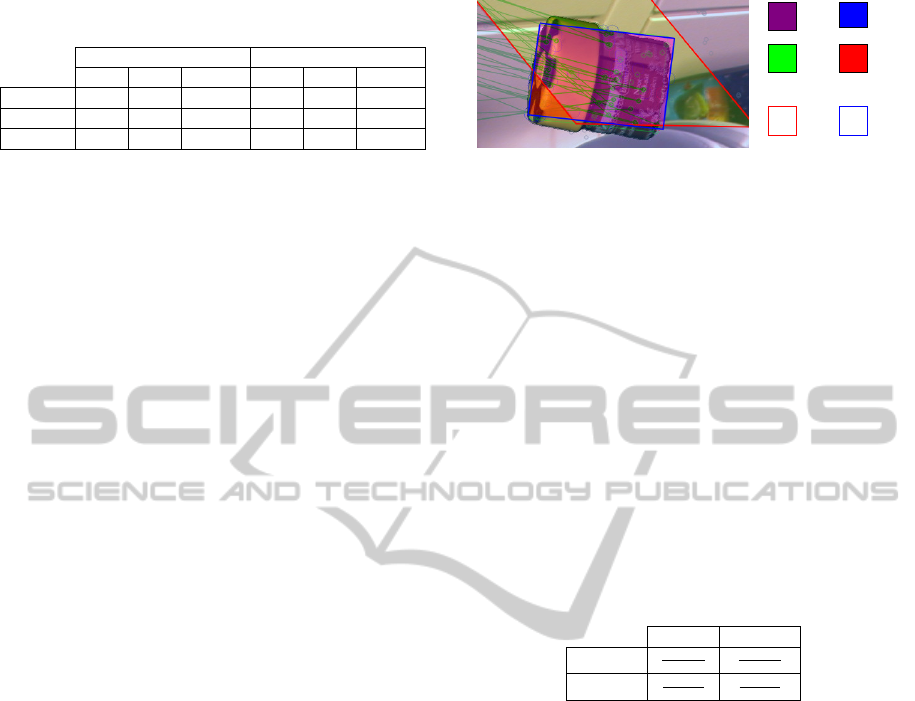
Table 1: Sum of n
ob j
i
, n
valid
i, j
and mean of c
i, j
, ¯c for the
textured and non-textured object set.
textured non-textured
SIFT form SIFText SIFT form SIFText
n
ob j
5093 6312 12054 3720 248 5992
n
valid
3973 4622 10044 2450 1943 4844
¯c [%] 78 73 83 66 78 81
MSER and ART as a descriptor (form) and the archi-
tecture, which is proposed in this paper. The sums of
n
ob j
i
, n
valid
i, j
and the mean of c
i, j
, which were obtained
during this experiment, are shown in table 1.
The number of detected features by SIFText is
significantly higher than the number of features ex-
tracted by each partial descriptor. Furthermore the
number of correct correspondences, obtained by em-
ploying SIFText, exceeds the sum of those generated
using the other descriptors. This increase is based on
the weighted combination of the descriptor parts and
would be lost, if a simple thresholding operation was
used instead. Moreover, the values of c calculated on
the textured and non-textured data set, while using
SIFText, are almost identical. This implies that the
descriptor’s performance is similar for both datasets;
hence it can be utilized effectively for the description
of textured and non-textured objects.
4.3 Matching Algorithm Evaluation
Considering the beforementioned ambiguity (cf. sec-
tion 3) a second test was proposed, which is able to
determine the accuracy of the calculation of an ob-
ject’s position and orientation in an image. According
to the procedure described in section 4.1 and 4.2 two
test images are created. For each test image
ˆ
I
i
a set of
features F
i
is extracted. Based on two sets of features
F
i
and F
j
an algorithm akin to the algorithm proposed
in chapter 3 is applied, yielding a transformation ma-
trix
ˆ
T
i,j
. By using equation 25, a subset of features
F
ob j
i
= {f
n
∈ F
i
: b
n
= 1} is obtained for each image
ˆ
I
i
, consisting of the features, which are located at the
object’s location in said image. For each set of features
F
ob j
i
the corresponding oriented bounding box B
i
is
calculated and transformed by
ˆ
T
i,j
and T
j,i
, yielding
ˆ
B
i
and
˜
B
i
. By intersecting the polygons defined by
ˆ
B
i
and
˜
B
i
the area of the intersection, A
t p
is obtained:
A
t p
= ||
˜
B
i
∩
ˆ
B
i
||. (30)
This area represents the portion of the object, which is
correctly transformed. The areas A
f p
and A
f n
in which
only one polygon exists, and thus are falsly matched,
are obtained, using the area
˜
A
i
and
ˆ
A
i
of
˜
B
i
and
ˆ
B
i
A
t p
A
f p
A
tn
A
f n
˜
B
i
B
i
Figure 9: Geometrical interpretation of A
t p
, A
f p
, A
tn
and
A
f n
, based on B
i
and
˜
B
i
.
respectively:
A
f p
=
˜
A
i
−A
t p
(31)
A
f n
=
ˆ
A
i
−A
t p
. (32)
The portion of the image that is correctly labeled as
background A
tn
is calculated according to equation 33
using the area of the whole test image A
image
:
A
tn
= A
image
−A
t p
−A
f p
−A
f n
. (33)
A geometrical representation of these calculations
is given by figure 9.
Based on the values of A
t p
, A
f p
, A
tn
and A
f n
con-
fusion matrices were created for the textured and non-
textured datasets utilizing a variety of combinations of
descriptor and matching algorithms according to the
following scheme:
object background
object
A
t p
A
t p
+A
f p
A
f p
A
t p
+A
f p
background
A
f n
A
tn
+A
f n
A
tn
A
tn
+A
f n
Values on the principal diagonal approaching 1 indi-
cate a nearly perfect result, while values close to 0
suggest that the object is detected at the wrong loca-
tion. The resulting confusion matrices are presented
in figures 10 and 11.
In figure 10 the performance of SIFT and SIFText
is similar for small values of K , if the experiment
is conducted on the textured dataset. Increasing K
yields no significant rise in the precision if SIFT is
used, while utilizing SIFText significantly increases
the value. The afore-mentioned ambiguities are solved,
by considering a higher amount of neighbours and the
performance is greatly increased. If the non-textured
dataset is used, SIFText clearly outperforms SIFT re-
gardless of K . In figure 11 very low precision values
are present. Since the background takes up the major-
ity of the image, a correct transformation matrix cannot
be deducted from the preponderance of the features.
RANSAC isn’t suited to be employed in this kind of
experiment. Nevertheless this experiment shows that
SIFText outperforms SIFT using both datasets.
DetectionofLow-texturedObjects
271

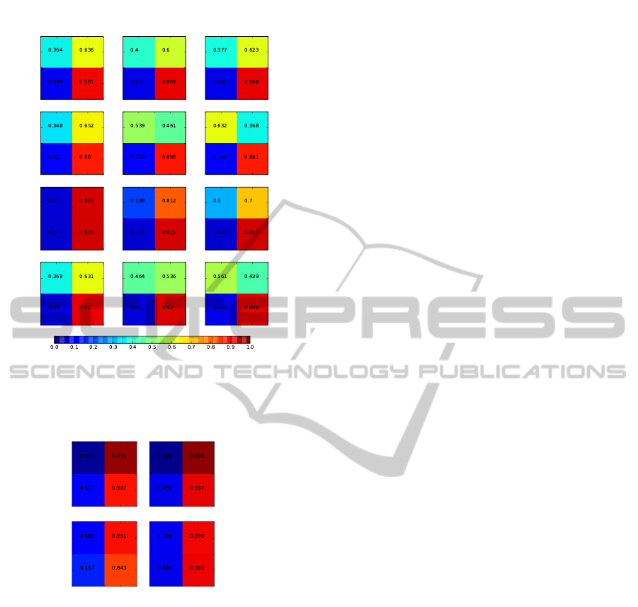
K = 2 K = 4 K = 6
SIFTSIFTextSIFTSIFText
texturednon-textured
Figure 10: Confusion matrices generated using the algorithm
proposed in chapter 3, for various values of the parameter K .
As descriptor algorithm SIFT and SIFText were used.
textured non-textured
SIFTSIFText
Figure 11: Confusion matrices generated using RANSAC
to calculate the homography. As descriptor algorithm SIFT
and SIFText were used. The color coding is the same used
in figure 10.
5 CONCLUSIONS
In this paper we have implemented and tested a de-
scriptor architecture, which was designed to detect
non-textured objects as well as textured objects, by
combining edge, shape and color description tech-
niques and weighting them by a locally calculated
value, derived from the texture of the image. Further-
more, a matching algorithm was implemented, that
was designed to mitigate the weak points of the de-
scriptor. In table 1 we have shown that for each object
the number of detected features was increased signifi-
cantly compared to SIFT, while the number of correct
correspondences was increased as well. This applies
to both, the textured and non-textured dataset. We
have further shown, that the precision of detecting
an object’s position and orientation in two images is
increased compared to RANSAC, if the matching al-
gorithm, which was developed here, is used (cf. figure
10 and 11). But even in the case RANSAC is used, the
descriptor surpasses SIFT.
By choosing the weighting factor locally and
adapting the descriptor accordingly features that were
matched incorrectly by the partial descriptors are as-
signed correctly. This architecture is, therefore, well
suited to detect textured and non-textured objects, as
well as objects, that possess textured and non-textured
parts.
REFERENCES
Bay, H., Tuytelaars, T., and van Gool, L. (2006). SURF:
Speeded Up Robust Features. Computer Vision ECCV
2006, 3951:404–417.
Bober, M. (2001). Mpeg-7 visual shape descriptors. Circuits
and Systems for Video Technology, IEEE Transactions
on, 11(6):716–719.
Bulla, C. and Hosten, P. (2013). Detection of false feature
correspondences in feature based object detection sys-
tems. In Proceedings of International Conference on
Image and Vision Computing New Zealand, Wellington,
New Zealand.
Fischler, M. A. and Bolles, R. C. (1981). Random sample
consensus: A paradigm for model fitting with appli-
cations to image analysis and automated cartography.
Commun. ACM, 24(6):381–395.
Forssen, P.-E. and Lowe, D.G. (2007). Shape descriptors
for maximally stable extremal regions. In Proceedings
of IEEE 11th International Conference on Computer
Vision, pages 1–8.
Geusebroek, J.-M., Burghouts, G.J., and Smeulders, A.W.M.
(2005). The amsterdam library of object images. Inter-
national Journal of Computer Vision, 61(1):103–112.
Ljubisa, M. and Sladjana, S. (2006). Orthonormal decompo-
sition of fractal interpolating functions. Series Mathe-
matics and Informatics, 21:1–11.
Lowe, D.G. (2004). Distinctive Image Features from Scale-
Invariant Keypoints. International Journal of Com-
puter Vision, 60(2):91–110.
Matas, J., Chum, O., Urban, M., and Pajdla, T. (2004).
Robust wide-baseline stereo from maximally stable
extremal regions. Image and Vision Computing,
22(10):761 – 767.
Naik, S. and Murthy, C. A. (2007). Distinct multicolored
region descriptors for object recognition. IEEE Trans-
actions on Pattern Analysis and Machine Intelligence,
29(7):1291–1296.
Tombari, F., Franchi, A., and Di Stefano, L. (2013). Bold
features to detect texture-less objects. In Proceedings
VISAPP2015-InternationalConferenceonComputerVisionTheoryandApplications
272

of IEEE International Conference on Computer Vision,
pages 1265–1272.
Toshev, A., Taskar, B., and Daniilidis, K. (2012). Shape-
based object detection via boundary structure segmen-
tation. International Journal of Computer Vision,
99(2):123–146.
Van De Weijer, J. and Schmid, C. (2006). Coloring local
feature extraction. In Proceedings of the 9th European
Conference on Computer Vision - Volume Part II, pages
334–348.
DetectionofLow-texturedObjects
273