
Time Series Modelling with Fuzzy Cognitive Maps
Study on an Alternative Concept’s Representation Method
Wladyslaw Homenda
1,2
, Agnieszka Jastrzebska
1
and Witold Pedrycz
3,4
1
Faculty of Mathematics and Information Science, Warsaw University of Technology,
ul. Koszykowa 75, 00-662 Warsaw, Poland
2
Faculty of Economics and Informatics in Vilnius, University of Bialystok, Kalvariju G. 135, LT-08221 Vilnius, Lithuania
3
System Research Institute, Polish Academy of Sciences, ul. Newelska 6, 01-447 Warsaw, Poland
4
Department of Electrical & Computer Engineering, University of Alberta, Edmonton, T6R 2G7 AB, Canada
Keywords:
Fuzzy Cognitive Map, Time Series Modelling and Prediction, Fuzzy Cognitive Map Design.
Abstract:
In the article we have discussed an approach to time series modelling based on Fuzzy Cognitive Maps (FCMs).
We have introduced FCM design method that is based on replicated ordered time series data points. We
named this representation method history h, where h is number of consecutive data points we gather. Custom
procedure for concepts/nodes extraction follows the same convention. The objective of the study reported in
this paper was to investigate how increasing h influences modelling accuracy. We have shown on a selection
of 12 time series that the higher the h, the smaller the error. Increasing h improves model’s quality without
increasing FCM’s size. The method is stable - gains are comparable for FCMs of different sizes.
1 INTRODUCTION
Fuzzy Cognitive Maps are fairly popular knowledge
representation scheme based on weighted directed
graphs. Nodes in the graph represent phenomena, arcs
represent relations. Among many fields of applica-
tion, FCMs are used to model time series.
Time series processing with FCMs has a substan-
tial advantage over classical approaches. FCMs op-
erate on the level of concepts, which are informa-
tion granules. Classical methods are based on scalars.
Concepts are higher-level interface for the underlying
information. They are introduced to facilitate supe-
rior human-machine interactions. Concepts in FCMs
are typically realized as a pair of a linguistic descrip-
tion and a fuzzy set. To cover the same fragment of
knowledge we either propose a few general concepts
or many specific concepts. The level of granulation
depends on the modelling objective. General con-
cepts form smaller models, knowledge is highly ag-
gregated. Such models are easier to interpret and to
use, but at the same time they are less precise in a nu-
merical context. In contrast, many specific concepts
produce larger model. Hence, predictions are more
accurate, but we may loose ease of interpretation.
We would like to emphasize that the goal of
time series modelling with FCMs is to offer human-
centered models. We take advantage of concepts-
based information representation scheme to describe
complex phenomena in as intuitive as possible way.
Study presented in this paper is focused on FCM
design procedure for time series modelling. In our
previous works we have discussed a general approach
to FCM design, and here we investigate its crucial el-
ement: time series representation. The objective of
our research was to experimentally test how increas-
ing time span represented by concepts would influ-
ence modelling quality. The research discussed in this
paper aims at improvement of FCM design so that one
can achieve higher precision and maintain model’s in-
tuitiveness and ease of interpretation at the same time.
Proposed FCM-based time series modelling is
novel and not yet present in the literature.
The article is structured as follows. Section 2 sum-
marizes relevant research to be found in the literature.
Section 3 presents developed methods. Section 4 con-
tains a description of experiments’ results. Section 5
covers conclusion and future research directions.
2 LITERATURE REVIEW
The research on FCMs has its beginnings in 1986,
when B. Kosko published his work in (Kosko, 1986).
406
Homenda W., Jastrzebska A. and Pedrycz W..
Time Series Modelling with Fuzzy Cognitive Maps - Study on an Alternative Concept’s Representation Method.
DOI: 10.5220/0005207704060413
In Proceedings of the International Conference on Agents and Artificial Intelligence (ICAART-2015), pages 406-413
ISBN: 978-989-758-074-1
Copyright
c
2015 SCITEPRESS (Science and Technology Publications, Lda.)

FCMs are present in sciences for 30 years now, how-
ever, their application to time series modelling has
been in the scope of interest for less than a decade.
There are three distinct approaches to time series
modelling with FCMs considered in the literature.
First, and most commonly studied one has been in-
troduced by W. Stach, L. Kurgan, and W. Pedrycz in
(Stach et al., 2008) in 2008. Cited work introduced
FCM design method for time series modelling based
on:
• time series representation as a sequence of pairs:
amplitude, change of amplitude,
• scalar time series fuzzification and extraction of
concepts that represent (fuzzified) time series val-
ues; concepts directly correspond to nodes in the
FCM,
• real-coded genetic algorithms for FCM training.
Summarized research has been an inspiration for fur-
ther attempts in this area. Examples of articles pre-
senting a research in the same direction are: (Lu et al.,
2013) and (Song et al., 2010).
Second approach to time series modelling with
FCMs has been brought up by W. Froelich and
E. I. Papageorgiou (Froelich et al., 2012; Froelich and
Papageorgiou, 2014). Proposed method is dedicated
to multivariate time series. In this approach FCM’s
nodes correspond to variables of the time series.
Third method has been introduced by the authors
in (Homenda et al., 2014b). This approach is based
on moving window technique. Nodes in a FCM are
ordered and they represent consecutive time points.
In this article we follow the approach introduced
in (Stach et al., 2008). Common elements of our and
cited method are: fuzzy concepts, fuzzification of ob-
servations into membership values. What is different:
time series and concepts representation method and
application of FCM simplification. We also use dif-
ferent training procedure, but this is only a technical
part of the modelling process.
3 DESIGNING FUZZY
COGNITIVE MAPS FOR TIME
SERIES MODELLING
The objective of the research on the application of
FCMs to time series modelling is to propose a design
technique that will extract interpretable nodes and
provide necessary training data to train the weights’
matrix.
Methods developed and investigated for this arti-
cle are related to the original approach introduced in
(Stach et al., 2008). In general, the proposed approach
and experiments on time series modelling with FCMs
could be decomposed into the following phases:
1. Time series conceptual representation.
2. FCM training.
3. Time series prediction (on a conceptual level).
3.1 Time Series Representation for
Modelling with Fuzzy Cognitive
Maps
Typically, a time series we process is not in concep-
tual form, but in scalar uni- or multivariate form. The
reason is that we often use instruments, such as ther-
mometers, seismometers, etc. to report current states
of phenomena. Conceptual knowledge repositories
are not available at all. This is why first we discuss
an algorithmic model for transforming any scalar time
series to conceptual one.
Proposed method is valid for both multi- and uni-
variate time series. Here for illustration purposes we
use univariate ones.
Let us denote a scalar time series as below:
a
1
,a
2
,a
3
,...,a
M
, where a
i
∈ R for i = 1,2,...,M
The sequence above is the most basic representa-
tion scheme for a time series. In our model we use
repeated historical data points scheme, which we call
history h, h ∈ N, h 6 M. Depending on the time span
h, elements of the original time series get repeated
with preservation of their order. For example:
• for history 2 time series is represented as follows:
(a
2
,a
1
),(a
3
,a
2
),(a
4
,a
3
),...,(a
M
,a
M−1
)
• for history 3 time series is represented as follows:
(a
3
,a
2
,a
1
),(a
4
,a
3
,a
2
),...,(a
M
,a
M−1
,a
M−2
)
And so on. Each element from the time series is re-
peated h times (the only exception is for first h − 1 el-
ements). This time series representation model does
not pre-process the original time series. It just repeats
already available information. In contrast, method
proposed by W. Stach et al. is based on time series
representation with pairs of amplitude and change of
amplitude. Theoretically, Stach’s et al. approach is
equivalent to history 2, but in our previous research
(Homenda et al., 2014a) we have shown that in prac-
tise unprocessed time series values are better: they
give models of higher accuracy and are easier to in-
terpret.
The greater the h, the more complex time series
representation. Let us take a closer look at h = 3
(history 3). Such model is very easy to interpret for
TimeSeriesModellingwithFuzzyCognitiveMaps-StudyonanAlternativeConcept'sRepresentationMethod
407

a human being. Each triple (a
i−2
,a
i−1
,a
i
) is inter-
preted as (day before yesterday, yesterday, today) if
the interval for gathering information was a day. In
general, history 3 is describing triples of (before be-
fore, before, now) data points. In comparison, Stach’s
et. al method in its generalized equivalent would
be representing the time series as triples of: (am-
plitude, change of amplitude, change of amplitude
change). The higher the h, the less straightforward
Stach’s model gets, while the method investigated in
this paper still maintains its transparency and is easy
to interpret.
Note that a time series represented with the his-
tory h model for h = 1,2,3 can be plotted in 1-,2-,3-
dimensional coordinates systems respectively. h can
be treated as the number of system’s dimensions.
Figure 1 illustrates an exemplar real-world time
series named Kobe in 1-dimensional space in time
(first plot), in 2-dimensional space of present and past
(middle image), and in 3-dimensional space of cur-
rent, past and before past. Kobe time series is publicly
available in a repository under (Hyndman, 2014).
3.2 Extraction of Concepts
Let us now discuss a method for elevation of a scalar
time series to a higher abstract level of concepts.
We aid ourselves, similarly as W. Stach et al., with
Fuzzy C-Means algorithm. The objective is to pro-
pose c concepts that generalize the time series. In
our procedure it is enough to perform it once, be-
cause selected time series representation scheme uses
repeated, but unprocessed values. For Stach’s et al.
method it is necessary to perform it h times. The aim
of applying Fuzzy C-Means to the original time series
a
0
,a
1
,... is to detect c clusters’ centers that become
concepts’ centres. Concepts describe in a granular,
aggregated fashion numerical values of the time se-
ries. The value of c is determining model’s specificity.
The number of target concepts can be either up
to system’s designer or decided by appropriate proce-
dures. An example of such procedure is described in
(Pedrycz and de Oliveira, 2008). Accuracy of clus-
tering into concepts is a very important factor. On
the other hand, the value of c is directly influencing
model’s complexity. High values of c produce large
and harder to interpret models. FCM-based model’s
quality is first of all judged by it’s ease of interpreta-
tion and application.
Concepts generalize values of the time series. The
choice of concepts is followed by a selection of appro-
priate linguistic variables that are attached to them.
Here are examples of linguistic variables: Small,
High, Small Negative, Moderately High, etc. For
convenience we usually abbreviate them and use only
first letters of each word. Linguistic variables enhance
the model and provide intuitive interface for its final
users - humans.
In our previous research we have investigated the
issues of the balance between specificity and general-
ity of the model. We have shown that to some extent
it depends on the character of a time series. In this
paper for comparability we assume c = 3 in all exper-
iments and attach the following linguistic variables:
Small (S), Moderate (M), High (H). Other values of
c are not considered here, because the main focus is
on time series representation. c = 3 was selected, be-
cause of its simplicity.
Moreover, Fuzzy C-Means not only extracts con-
cepts’ centres, but also provides a formula for calcu-
lating membership levels (u) to proposed concepts:
u
i j
=
1
c
∑
k=1
||a
i
− v
j
||
||a
i
− v
k
||
2/(m−1)
(1)
u
i j
is a membership value of i-th data point to j-
th concept. c is the number of clusters-concepts,
so j = 1,...,c. Data points in this context match
time series representation scheme. Data points are
denoted as a
i
= [a
i+h−1
,...,a
i
],i = 1, . . . , M − h + 1,
where M is the length of the input scalar time series.
v
j
= [v
j1
,...,v
jh
] describes j-th concept. m is fuzzifi-
cation coefficient (m > 1), ||·|| is the Euclidean norm,
On the output of Fuzzy C-Means procedure we
obtain 1-dimensional concepts’ centres. To adapt
them to the time series representation scheme we have
to elevate them to h-dimensional space by applying
h-nary Cartesian product. This results in c
h
new h-
dimensional concepts.
Again, with the use of Formula 1 we calculate
membership levels of time series data points to new
concepts. This time the number of concepts is not c,
but c
h
.
Concepts and values of corresponding member-
ship levels for time series data points provide all nec-
essary information to train a FCM. Extracted concepts
become nodes in FCM. Training data are levels of
membership, which during the process of FCM learn-
ing are passed to appropriate nodes.
Proposed method for FCM design purposefully
extracts a lot of concepts. We apply Cartesian prod-
uct, so we suspect that not all of the proposed con-
cepts reflect the underlying time series. We may eval-
uate quality of a concept v
j
by calculating its mem-
bership index M(v
j
):
M(v
j
) =
N
∑
i=1
u
i j
(2)
ICAART2015-InternationalConferenceonAgentsandArtificialIntelligence
408

Figure 1: Kobe time series and its representation in: history 1 (left plot), history 2 (middle plot), and history 3 (right plot).
N is the size of training data. Training data is a subset
of all available data used in FCM design and training.
The remainder data subset is called test and it is for
evaluation of the proposed model.
Membership index informs how strongly a con-
cept represents the time series. M(v
j
) is a sum of
membership values of all data points to concept j.
Weak values of membership index say that given con-
cept is weakly tied to the dataset. Strong values of
membership index indicate that the concept is able to
represent time series well.
In the process of further model tuning one may
decide to get rid of weak nodes. Hence, we introduce
letter n to describe the final number of concepts in
the model. Membership index can be used to sepa-
rate good nodes from bad ones. We call this proce-
dure FCM simplification as its objective is to make
the model smaller. In this paper we present a series
of experiments, where we apply membership index to
obtain FCMs of desired size.
3.3 Learning Procedure
FCMs represent relations within knowledge. FCM
size - the number of its nodes is denoted as n. FCMs
are illustrated with weighted directed graphs. The
core of each FCM is its weights’ matrix denoted
as W = [w
i j
],w
i j
∈ [−1,1],i, j = 1,...,n. Weights
describe relations between modelled phenomena.
Though fuzzy sets are associated with the [0,1] do-
main, weights values span onto the whole [−1, 1] do-
main. In this way we are able to represent negative
relations. Weights that are evaluated as 0 mean that
there is no relation between two concepts. In the case
of the proposed time series modelling scheme, nodes
in the FCM are equivalent to concepts. Hence, nodes
represent concepts that generalize values of the time
series.
FCM training procedure aims at optimizing
weights matrix W. The weights matrix learning pro-
cedure’s objective is to minimize differences between
predictions provided by the FCM and real, target val-
ues of conceptualized time series.
FCM exploration is by the following formula:
Y = f (W · X) (3)
where f is a sigmoid transformation function:
f (t) =
1
1 + exp(−τt)
(4)
Value of parameter τ was set to 5 based on experi-
ments and literature review: (Mohr, 1997; Stach et al.,
2008).
In the input layer of the FCM-based model we
have activations (X = [x
ji
],x
ji
∈ [0,1], j = 1,...,n,i =
1,...,N). N is the number of available training
data. Single activations vector is denoted as x
i
=
[x
1i
,x
2i
,...,x
ni
] and it concerns i-th data point a
i
. In
the FCM exploration process, activations are passed
to FCM nodes.
In the output layer of FCM-based model we have
FCM responses denoted as Y = [y
ji
],y
ji
∈ [0,1], j =
1,...,n,i = 1,...,N. FCM responses model and pre-
dict phenomena of interest. Hence, the quality of
given FCM is assessed with discrepancies between
FCM responses Y and goals G.
Goals matrix G = [g
ji
],g
ji
∈ [0,1] is of size n × N
and it gathers actual, reported states of n nodes, N is
the number of training data.
FCM learning procedure iteratively adjusts
weights matrix, so that the aforementioned discrep-
ancies are minimized. Typically, objective function
is Mean Squared Error (MSE) between FCM outputs
and goals:
MSE =
1
n · N
·
N
∑
i=1
n
∑
j=1
(y
ji
− g
ji
)
2
(5)
In the literature one may find many articles de-
voted to FCMs learning. Since this is not the subject
of this paper we do not discuss this research to greater
extent here, just give references to selected papers on
TimeSeriesModellingwithFuzzyCognitiveMaps-StudyonanAlternativeConcept'sRepresentationMethod
409

different approaches: (Papageorgiou et al., 2003; Par-
sopoulos et al., 2003; Stach et al., 2005). In our exper-
iments we train FCMs with the use of PSO, with its
implementation in R available in ”pso” package. All
arguments were left to default Standard PSO 2007,
full list is under (Bendtsen, 2014).
4 EXPERIMENTS
4.1 Study Objectives and Methods
The focus of this paper is on the proposed time series
representation scheme, named history h. The objec-
tive of our study is to investigate how increasing the
length of time span (h) represented by concepts im-
proves modelling accuracy. We are especially inter-
ested if there is any differences in gains for small and
large FCMs.
In order to address named issues we have set up
a series of experiments. We have investigated 3 syn-
thetic and 9 real-world time series. Synthetic time
series were constructed based on a fixed base of num-
bers that constitute their period. Base sequence was
replicated so that the total length of the input time se-
ries is 3000. Next, we added a noise: to each time
series scalar data a random value from a normal dis-
tribution having a mean of 0 and a standard deviation
of 0.7. In further parts of this article we name synthe-
sised time series by their base sequence.
Real-world time series were downloaded from
a publicly available repository under (Hyndman,
2014). Names of real-world time series in this arti-
cle are the same as in the cited database. Selected
time series were of significantly different properties.
Due to space limitations we do not elaborate on their
characteristics. The aim of using both synthetic and
real-world time series was to thoroughly test the pro-
posed time series representation scheme. Synthetic
time series are very regular, while real-world datasets
are not.
The results presented in this paper are a selection
of an extensive series of experiments on more time se-
ries. Due to space limitations we use just 12 datasets
to illustrate our approach, results of other tests were
consistent with the ones discussed here.
In the course of the experiments we have used first
70% of data points for FCM learning, remaining 30%
were for predictions only. First part is called train,
second test set. Experiments were for FCMs of differ-
ent sizes: n = 4,6,8,10,12,17,22,27. For each case
we have tested history 3, history 4, and history 6 rep-
resentation schemes.
Note that in order to compare results of the three
time series representation methods maps had to be
of the same size. Therefore, we have applied mem-
bership index to remove appropriate number of worst
nodes from models that were originally large. Mod-
els obtained with history 3 method were originally
of size 3
3
= 27. Models with history 4 were of size
3
4
= 81. Models with history 6 had initially 3
6
= 729
concepts. The largest of trained maps had n = 27
nodes, which is a lot, but still manageable to train
and apply. Large models are impractical to train and
to apply. Let us remind that the number of weights
for optimization is the number of concepts squared,
but time necessary to train such FCM grows much
faster than quadratically. Therefore, we have deter-
mined that n = 27 is one of largest reasonable FCM.
Its weights matrix requires around 3-4 days to opti-
mize with a single-threaded process on a standard PC.
As a measure of quality we use MSE, which has
been also the objective function for optimization pro-
cedure. Figure 2 illustrates MSE for 3 synthetic and
9 real-world time series. Chart is ordered according
to FCM size. Names of time series are in plots, the
following abbreviations are used: h3 for history 3, h4
for history 4, and h6 for history 6.
4.2 Results
The accuracy of modelling depends on map size. The
larger the map, the smaller the MSE. This observa-
tion comes with no surprise though. In large maps
concepts generalize smaller fragment of information.
In contrast, small maps, like n = 4 are based on gen-
eral concepts that have to represent greater part of the
time series, hence model’s accuracy is worse.
Proposed time series representation scheme al-
lows to increase the accuracy of models without in-
creasing FCM size. In each case the greater h, the
smaller the MSE for FCMs of the same size. MSEs
on conceptualized real-world time series are typically
lower than on synthetic time series. Observe, that the
OY scale for the best fitted models is to 0.004. Errors
for four such time series: Synthetic-258, DailyIBM
(stocks), Equiptemp (temperature of lab equipment),
Wave2 (frequency of waves) are very small. For the
DailyIBM time series errors were so small that the
bars are hardly visible in used scale.
In Figure 2 we see that for smaller maps, like n = 4
and n = 6, increasing h resulted in greater improve-
ment than for large maps. This is natural consequence
of the fact that errors on smaller maps were higher at
start, so we can improve them more.
It is worth to notice, that errors on predictions
(test) are very close to errors on training data. Test
ICAART2015-InternationalConferenceonAgentsandArtificialIntelligence
410

Figure 2: MSE for 3 synthetic and 9 real-world fuzzified time series for FCM-based models with different number of nodes
(4, 6, ..., 27) and different time series representation schemes: h3 stands for history 3, h4 for history 4 and h6 for history 6.
predictions were for data points that were not in-
cluded in the training dataset.
Let us now investigate the gain of accuracy
achieved by applying time series representation
scheme with larger h. Figure 3 illustrates the gain in
MSE achieved by increasing value of h from 3 to 4
(lighter bars) and from 3 to 6 (darker bars).
Plots in Figure 3 show percentage increase of
modelling accuracy. Gains were calculated based on
a percentage decrease of MSE, achieved when we in-
crease h. We have used the following formula:
Gain
h+d
=
MSE
h
− MSE
h+d
MSE
h
· 100% (6)
Gain
h+d
informs about a percentage decrease of MSE
when we increase the time span from h to h + d. Neg-
ative values of Gain inform that there was no increase
at all. The larger the Gain, the more MSE dropped by
TimeSeriesModellingwithFuzzyCognitiveMaps-StudyonanAlternativeConcept'sRepresentationMethod
411
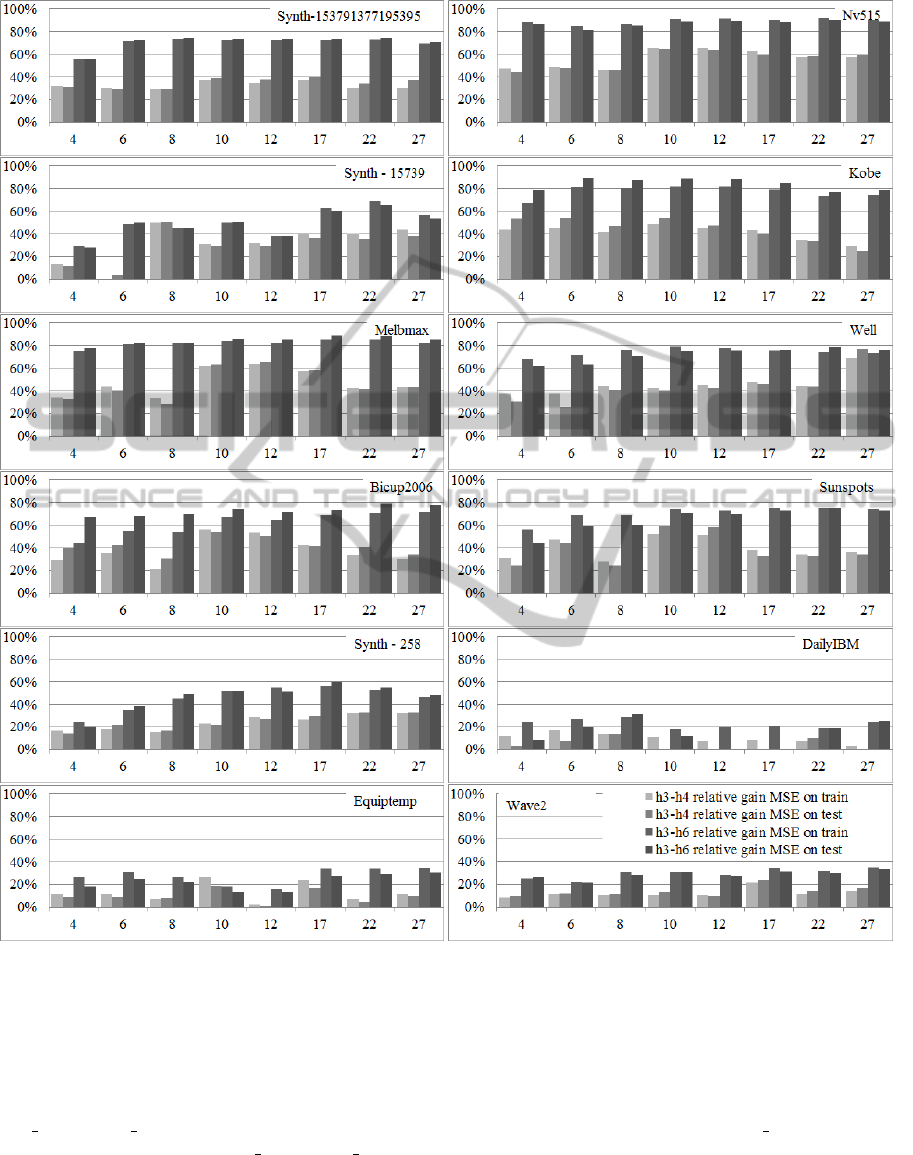
Figure 3: Percentage gain of accuracy on train and test sets achieved by increasing the time span: from h = 3 to h = 4 pale
grey bars, and from h = 3 to h = 6 dark grey bars.
increasing time span.
The more we increase the time span coded in con-
cepts, the higher accuracy we achieve. In Figure 3
lighter bars that correspond to the upgrade from his-
tory 3 to history 4 are smaller than darker ones plot-
ted for the upgrade from history 3 to history 6.
The gain is comparable for FCMs of all sizes.
Small FCMs can be equally well improved as large
ones. This is especially appealing property. By in-
creasing h we are able to achieve better results for
very small models without increasing their size.
The gain is different for different time series.
For three time series that were modelled with very
high precision at start (for history 3): DailyIBM,
Equiptemp, and Wave2 the improvement is lower than
for the other time series.
To sum up, the proposed time series representa-
tion method improves modelling quality. Typically,
ICAART2015-InternationalConferenceonAgentsandArtificialIntelligence
412

increasing the time span for concepts from h = 3 to
h = 4 improves modelling accuracy by circa 40%,
while increasing the time span from h = 3 to h = 6
improves it by circa 80%.
5 CONCLUSIONS
Proposed time series and concepts’ representation
method for time series modelling with FCMs is based
on gathering h consecutive elements of the input time
series into a single data point. The larger the h, the
longer time span is captured in a single data point and
in extracted concepts. Empirical studies show that ap-
plying this method is beneficial. It allows to increase
modelling accuracy without increasing FCM size.
We have shown that long time spans (like h = 6)
bring higher numerical accuracy, but in our opinion
for a model that would be used by humans h = 3
or 4 are reasonable values. The larger h, the more
computationally demanding is the modelling process.
The allocation of a matrix for membership values is
memory-demanding, while optimization of weights
matrix is time-demanding.
Most important advantage of the proposed method
is transparency of time series and concepts represen-
tation method. Each data point in our model has the
same interpretation and it represents an h-long time
span. Information is not processed and, if necessary,
can be translated in a straightforward way back to the
numeric time series.
In future research we will address interpretation
issues of trained FCMs. We will also take under fur-
ther investigation FCM training procedure.
ACKNOWLEDGEMENTS
The research is partially supported by the Foundation
for Polish Science under International PhD Projects
in Intelligent Computing. Project financed from The
European Union within the Innovative Economy
Operational Programme (2007- 2013) and European
Regional Development Fund.
The research is partially supported by the National
Science Center, grant No 2011/01/B/ST6/06478.
REFERENCES
Bendtsen, C. (2014). Package ’pso’. http://cran.r-
project.org/web/packages/pso/pso.pdf. [Online; ac-
cessed 14-November-2014].
Froelich, W. and Papageorgiou, E. (2014). Extended evolu-
tionary learning of fuzzy cognitive maps for the pre-
diction of multivariate time-series. In Fuzzy Cognitive
Maps for Applied Sciences and Engineering, pages
121–131.
Froelich, W., Papageorgiou, E., Samarinasc, M., and Skri-
apasc, K. (2012). Application of evolutionary fuzzy
cognitive maps to the long-term prediction of prostate
cancer. In Applied Soft Computing 12, pages 3810–
3817.
Homenda, W., Jastrzebska, A., and Pedrycz, W. (2014a).
Fuzzy cognitive map reconstruction - dynamics vs.
history. In Proceedings of ICNAAM, page in press.
Homenda, W., Jastrzebska, A., and Pedrycz, W. (2014b).
Modeling time series with fuzzy cognitive maps. In
Proceedings of the WCCI 2014 IEEE World Congress
on Computational Intelligence, pages 2055–2062.
Hyndman, R. (2014). Time series repository.
http://robjhyndman.com/tsdldata. [Online; accessed
14-November-2014].
Kosko, B. (1986). Fuzzy cognitive maps. In Int. J. Man
Machine Studies 7.
Lu, W., Yang, J., and Liu, X. (2013). The linguistic fore-
casting of time series based on fuzzy cognitive maps.
In Proc. of IFSA/NAFIPS, pages 2055–2062.
Mohr, S. (1997). The use and interpretation of fuzzy cogni-
tive maps. In Master’s Project, Rensselaer Polytech-
nic Institute.
Papageorgiou, E. I., Stylios, C. D., and Groumpos, P. P.
(2003). Fuzzy cognitive map learning based on non-
linear hebbian rule. In Australian Conf. on Artificial
Intelligence, pages 256–268.
Parsopoulos, K., Papageorgiou, E., Groumpos, P., and Vra-
hatis, M. (2003). A first study of fuzzy cognitive
maps learning using particle swarm optimization. In
Proc. IEEE 2003 Congr. on Evolutionary Computa-
tion, pages 1440–1447.
Pedrycz, W. and de Oliveira, J. V. (2008). A development
of fuzzy encoding and decoding through fuzzy clus-
tering. In Clustering, in IEEE Transactions on In-
strumentation and Measurement, Vol. 57, No. 4, pages
829–837.
Song, H., Miao, C., Roel, W., and Shen, Z. (2010). Im-
plementation of fuzzy cognitive maps based on fuzzy
neural network and application in prediction of time
series. In IEEE Transactions on Fuzzy Systems, 18(2),
pages 233–250.
Stach, W., Kurgan, L., and Pedrycz, W. (2008). Numeri-
cal and linguistic prediction of time series. In IEEE
Transactions on Fuzzy Systems, 16(1), pages 61–72.
Stach, W., Kurgan, L., Pedrycz, W., and Reformat, M.
(2005). Genetic learning of fuzzy cognitive maps. In
Fuzzy Sets and Systems 153, pages 371–401.
TimeSeriesModellingwithFuzzyCognitiveMaps-StudyonanAlternativeConcept'sRepresentationMethod
413
