
Wiener-Hopf Analysis of the Diffraction by a Finite Sinusoidal
Grating: The Case of H Polarization
Toru Eizawa and Kazuya Kobayashi
Department of Electrical, Electronic, and Communication Engineering, Chuo University,
1-13-27 Kasuga, Bunkyo-ku, Tokyo 112-8551, Japan
eizawa@mth.biglobe.ne.jp, kazuya@tamacc.chuo-u.ac.jp
Keywords: Wiener-Hopf technique, perturbation method, scattering and diffraction, finite sinusoidal grating.
Abstract: The diffraction by a finite sinusoidal grating is analyzed for the H-polarized plane wave incidence using the
Wiener-Hopf technique combined with the perturbation method. The scattered far field is evaluated with the
aid of the saddle point method, and scattering characteristics of the grating are discussed via numerical
examples of the far field intensity.
1 INTRODUCTION
The analysis of the diffraction by gratings is
important in electromagnetic theory and optics.
Various analytical and numerical methods have been
developed and the diffraction phenomena have been
investigated for many kinds of gratings (Ikuno and
Yasuura, 1973; Shestopalov et al., 1973; Hinata and
Hosono, 1976; Petit, 1980; Okuno, 1993).
The Wiener-Hopf technique is known as a
rigorous approach for analyzing wave scattering
problems related to canonical geometries, and can be
applied efficiently to the analysis of the diffraction by
specific periodic structures.
Most of the analyses in the relevant works done in
the past are restricted to periodic structures of infinite
extent and plane boundaries and hence, it is important
to investigate the problems without these restrictions.
In our previous paper, we have considered a finite
sinusoidal grating as an example of gratings of finite
extent and non-plane boundaries, and analyzed the E-
polarized plane wave diffraction based on the
Wiener-Hopf technique combined with the
perturbation method (Kobayashi and Eizawa, 1991).
This problem is important in investigating the end
effect of finite gratings as well as the applicability of
the Wiener-Hopf technique to obstacles with non-
plane boundaries.
In this paper, we shall consider the same grating
geometry as in Kobayashi and Eizawa (1991), and
analyze the diffraction problem for the H-polarized
plane wave incidence. Assuming that the corrugation
amplitude of the grating is small compared with the
wavelength, the original problem is approximately
replaced by the problem of the H-polarized plane
wave diffraction by a flat strip with a certain mixed
boundary condition. We also expand the unknown
scattered field using a perturbation series and separate
the diffraction problem under consideration into the
zero-order and the first-order boundary value
problems.
Introducing the Fourier transform for the
unknown scattered field and applying boundary
conditions in the transform domain, the problem is
formulated in terms of the zero- and first-order
Wiener-Hopf equations, which are solved exactly via
the factorization and decomposition procedure.
However, the solution is formal in the sense that
branch-cut integrals with unknown integrands are
involved. These branch-cut integrals are then
evaluated asymptotically for the width of the grating
large compared with the wavelength, leading to an
explicit high-frequency solution. Taking the Fourier
inverse of the solution in the transform domain and
applying the saddle point method, the scattered far
field in the real space is derived. Based on these
results, we have carried out numerical computation of
the far field intensity for various physical parameters.
Scattering characteristics of the grating are discussed
in detail via numerical examples.
The time factor is assumed to be e
-iωt
and
suppressed throughout this paper.
62
Eizawa T. and Kobayashi K.
Wiener-Hopf Analysis of the Diffraction by a Finite Sinusoidal Grating: The Case of H Polarization.
DOI: 10.5220/0005421300620067
In Proceedings of the Third International Conference on Telecommunications and Remote Sensing (ICTRS 2014), pages 62-67
ISBN: 978-989-758-033-8
Copyright
c
2014 by SCITEPRESS – Science and Technology Publications, Lda. All rights reserved
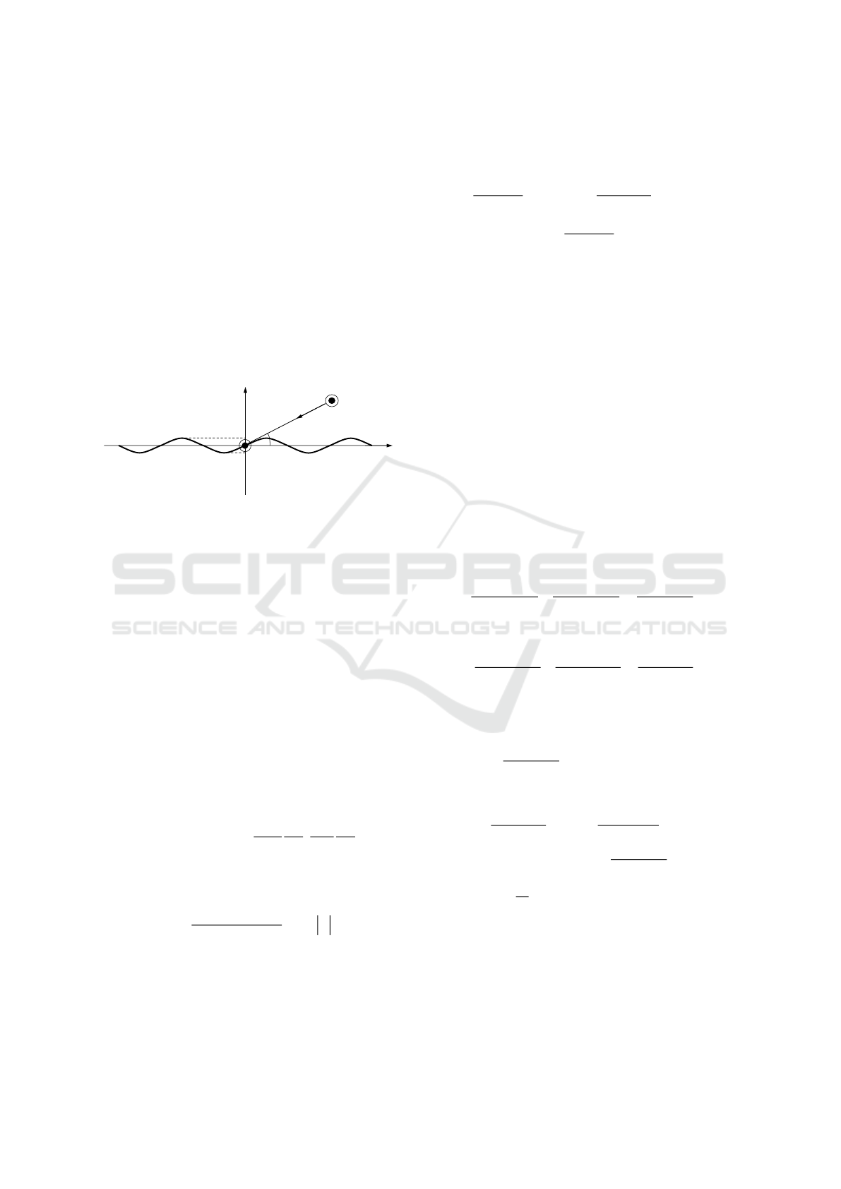
2 STATEMENT OF THE
PROBLEM
We consider the diffraction of an H-polarized plane
wave by a finite sinusoidal grating as shown in Fig.
1, where the grating surface is assumed to be
infinitely thin, perfectly conducting, and uniform in
the
-y
direction, being defined by
sin ( 0, 0)x h mz m h
(1)
for
|| .
za
In view of the grating geometry and the
characteristics of the incident field, this is a two-
dimensional problem.
Let us define the total magnetic field
(, )
t
xz
[ ( , )]
t
y
H xz
by
(, ) (, ) (, ),
ti
xz xz xz
(2)
where
(, )
i
xz
is the incident field of H polarization
given by
00
( sin cos )
(, )
ik x z
i
xz e
(3)
for
0
0 /2
with
1/2
00
[ ( )]k
being the
free-space wavenumber. The scattered field
(, )xz
satisfies the two-dimensional Helmholtz equation
2 2 2 22
( / / ) ( , ) 0.x z k xz
(4)
Once the solution of (4) has been found, nonzero
components of the scattered electromagnetic fields
are derived from the following relation:
00
1
(,,) , , .
yxz
i
HEE
iz x
(5)
According to the boundary condition, tangential
components of the total electric field
tan
t
E
satisfies
tan
( sin , )
0, ,
t
t
h mz z
E za
n
(6)
where
/ n
denotes the normal derivative on the
grating surface. We assume that the corrugation
depth
2h
is small compared with the wavelength,
and expand (6) in terms of a Taylor series around
0.x
Then by ignoring the
2
()Oh
terms from the
Taylor expansion, we obtain that
2
2
2
(0, ) (0, )
sin
(0, )
cos ( ) 0
tt
t
zz
h mz
x
x
z
m mz O h
z
(7)
for
|| .za
Equation (7) is the approximate
boundary condition used throughout the rest of this
paper.
We express the unknown scattered field
(,)xz
in terms of a perturbation series expansion in
h
as
(0) (1) 2
(,) (,) (,) ( ),xz xz h xz Oh
(8)
where
(0)
(,)xz
and
(1)
(,)xz
are the zero-order and
the first-order terms contained in the scattered field,
respectively. Substituting (8) into (4) and using (2),
(3), and (7), the original problem can be separated
into the two perturbation problems.
The zero-order and first-order scattered fields
()
(,)
n
xz
for
0,1n
satisfy
2 2 2 2 2 ()
( / / ) ( , ) 0,
n
x z k xz
(9)
where the boundary conditions are given by
(0) (0) (0)
( 0, ) ( 0, )[ (0, )],z zz
(10)
(0) (0) (0)
( 0, ) ( 0, ) (0, )
,
z zz
x xx
(11)
(1) (1) (1)
( 0, ) ( 0, ) (0, ) ,z zz
(12)
(1) (1) (1)
( 0, ) ( 0, ) (0, )z zz
x xx
(13)
for
|| ,za
and
(0) (0) (0)
( 0, ) ( 0, ) (0, ),z zj z
(14)
0
(0)
cos
0
(0, )
sin ,
ikz
z
ik e
x
(15)
(1) (1) (1)
( 0, ) ( 0, ) (0, ),z zj z
(16)
(1) 2 (0)
2
(0)
2
cos
2
0
1
2
cos
0
1
(0, ) (0, )
sin
(0, )
cos
sin ( 1)
2
cos
n
n
ikz
n
n
ikz
n
zz
mz
x
x
z
m mz
z
ik
ke
me
(17)
for
||za
with
1,2 0
cos cos / .mk
(18)
Figure 1: Geometry of the problem.
x
()
ii
y
H
h
h
y
a
a
0
z
Wiener-Hopf Analysis of the Diffraction by a Finite Sinusoidal Grating: The Case of H Polarization
63

In (14) and (16),
(0)
(0, )jz
and
(1)
(0, )jz
are the zero-
order and first-order terms of the unknown surface
currents induced on the grating surface, respectively.
As seen from the above discussion, the zero-order
problem corresponds to the diffraction by a perfectly
conducting flat strip. On the other hand, the first-
order problem is important since it contains the
effect due to the sinusoidal corrugation.
3 WIENER-HOPF EQUATIONS
For convenience of analysis, we assume that the
medium is slightly lossy as in
12
k k ik
with
21
0.kk
Using the radiation condition, it follows
from (8) that the zero- and first-order scattered fields
()
(,)
n
xz
for
0, 1
n
show the asymptotic behavior
20
| |cos
()
( , ) ( ), | | .
kz
n
x z Oe z
(19)
Let us introduce the Fourier transform of the
scattered field
()
(,)
n
xz
with respect to
z
as in
() 1/2 ()
(, ) (2) (, ) ,
n n iz
x x z e dz
(20)
where
Re Im ( ).ii
It follows
from (19) and (20) that
()
(, )
n
x
for
0, 1n
are
regular in the strip
20
| | cosk
of the complex
-
plane. We also introduce the Fourier integrals as
()
1/2
() ( )
( , ) (2 )
(,) ,
n
n i za
a
x
x z e dz
(21)
()
1/2 ( )
1
(, ) (2) (,) ,
a
n
n iz
a
x x z e dz
(22)
1/2
()
()
1
(0, ) 2 (0, ) .
a
n
n iz
a
J j z e dz
(23)
Then it is seen that
()
(, )
n
x
are regular in
20
cosk
whereas
()
1
(, )
n
x
and
()
1
(0, )
n
J
are
entire functions. It follows from (20)-(22) that
()
() ()
1
()
(, ) (, ) (, )
( , ).
n
n ia n
n
ia
xe x x
ex
(24)
Taking the Fourier transform of (9) and making
use of (19), we derive that
2 2 2 ()
[ / ( )] ( , ) 0,
n
d dx x
(25)
where
2 2 1/2
() ( )k
with
Re ( ) 0.
The
solution of (25) is expressed as
() () ()
() ()
( , ) ( ) , 0,
() , 0
n nx
nx
x Ae x
Be x
(26)
for
0, 1,n
where
()
()
n
A
and
()
()
n
B
are
unknown functions. Setting
0
x
in (26) and
arranging the results, we obtain that
() ()
() ()
( 0, ) ( 0, )
() (),
nn
nn
AB
(27)
() ()
() ()
( 0, ) ( 0, )
()[ () ()],
nn
nn
AB
(28)
where the prime denotes differentiation with respect
to
x
. Using the boundary conditions as given by
(10)-(17), (26) is now expressed as
(0) (0) ( )
1
( , ) (1 / 2) ( ) ,
x
x Je
(29)
(1) (1) ( )
1
12
(0)
1
2
(0) ( )
1
( , ) (1 / 2) ( )
[4 ( )] {[ ( ) ( )]
()
[()()]
( )]}
x
x
x Je
i mm m
Jm
mm m
J me
(30)
for
0x
. Equations (29) and (30) are the zero- and
first-order scattered fields in the Fourier transform
domain, respectively.
Setting
0x
in (29) and (30) and carrying
out some manipulations with the aid of the boundary
conditions, we are led to
(0)
1
()
() () (0,)
( ) 0,
ia
ia
e U KJ
eU
(31)
(1)
1
()
() () (0, )
() 0
ia
ia
eV K J
eV
(32)
for
20
| | cos ,k
where
0
(0)
0
( ) (0, ) ,
cos
A
U
k
(33)
(0)
0
()
0
( ) (0, ) ,
cos
B
U
k
(34)
2
1
() () (1) ,
cos
n
nn
n
n
AC
V
k
(35)
2
()
1
() () (1) ,
cos
n
nn
n
n
BC
V
k
(36)
() ()/2K
(37)
with
Third International Conference on Telecommunications and Remote Sensing
64

(1)
2
(0)
2
(0)
1/2 (0)
( ) (0, ) (1 / 2 )
{[()()]
(0, )
[()()]
(0, )
(2 ) cos (0, )},
ima
ima
i
mm m
em
mm m
em
m ma a
(38)
0
cos
0
0
1/2
0
sin
,
(2 )
ika
A
ke
B
(39)
cos
1/2
, 1, 2,
(2 )
n
ika
n
n
A
e
n
B
(40)
2
00
( / 2)[ sin ( 1) cos ],
1, 2.
n
n
C kk m
n
(41)
Equation (31) and (32) are the zero- and first-order
Wiener-Hopf equations, respectively.
4 EXACT AND ASYMPTOTIC
SOLUTIONS
In this section, we shall solve the zero- and first-
order Wiener-Hopf equations to obtain exact and
asymptotic solutions. First we note that the kernel
function
()K
is factorized as
() () (),K KK
(42)
where
()
K
are the split functions defined by
1/2 /4 1/2
() 2 ( ) .
i
K ek
(43)
Multiplying both sides of (31) by
/ ()
ia
eK
and applying the decomposition procedure with the
aid of the edge condition, we arrive at the exact
solution with the result that
()
0
00
() ()
( cos )( cos )
1
[ () ()],
2
sd
UK
B
Kk k
uu
(44)
0
00
() ()
( cos )( cos )
1
[() ()],
2
sd
UK
A
Kk k
uu
(45)
where
2,
()
.
()
1
() ,
( )( )
i a sd
ki
sd
k
eU
ud
iK
(46)
,
() ()
() () ().
sd
U UU
(47)
Equations (44) and (45) are formal since branch-cut
integrals with the unknown integrands
,
()
()
sd
U
are
involved. Applying a rigorous asymptotic method
developed by Kobayashi (2013), we obtain a high-
frequency solution explicitly as in
0
00
1 00
() ()
( cos )( cos )
( )[ ( ) ( )],
ub
UK
A
Kk k
KC B
(48)
()
0
00
2 00
() ()
( cos )( cos )
()[ () ()]
ua
UK
B
Kk k
KC A
(49)
for
,ka
where
1,2
22
,,
00
()
1 () ()
[ () ()() ()],
u
ab ba
Kk
C
Kk k
k Kk k k
(50)
1/2 2
1
2
( ) (1 / 2, 2 ( ) ),
ika
ae
i ka
(51)
,
0
0
0
( ) ( cos )
()
cos
ab
k
k
(52)
with
0 00 00
() () (),
aa b
A BP
(53)
0 00 00
() () (),
bba
B AP
(54)
,
0
0
0
1
()
cos
11
.
( ) ( cos )
ab
P
k
K Kk
(55)
In (51),
1
(, )
is the generalized gamma function
(Kobayashi, 1991) defined by
1
0
(,)
()
ut
m
m
te
u v dt
tv
(56)
for
Re 0,u
| | 0,v
| arg | ,v
and positive
integer
.m
This completes the solution of the zero-
order Wiener-Hopf equation (31).
Wiener-Hopf Analysis of the Diffraction by a Finite Sinusoidal Grating: The Case of H Polarization
65

A similar procedure may also be applied to the
first-order Wiener-Hopf equation (32). Omitting the
whole details, we arrive at a high-frequency solution
with the result that
2
1
cos
1/2
1/2 1/2
1
11 22
( ) ( 1)
()
(2 ) ( cos ) ( cos )
( )[ ( )
() ()],
n
n
n
ika
n
nn
v
bb
V
Ce k
k kk
KD
BB
(57)
2
()
1
cos
1/2
1/2 1/2
2
11 22
( ) ( 1)
()
(2 ) ( cos ) ( cos )
()[ ()
() ()]
n
n
n
ika
n
nn
v
aa
V
Ce k
k kk
KD
AA
(58)
as
,ka
where
1,2
22
2
,,
1
()
1 () ()
() ()() ()
v
ab ba
nn
n
Kk
D
Kk k
k Kk k k
(59)
and
,
( ) ( cos )
( ) ( 1) ,
cos
ab n
n
nn
n
k
C
k
(60)
() () (1) (),
a a nb
n nn n nn
A BC P
(61)
() () (1) (),
b b na
n nn n nn
B AC P
(62)
,
1
()
cos
11
( ) ( cos )
ab
n
n
n
P
k
K Kk
(63)
for
1, 2 .n
Equations (48), (49) and (57), (58)
yield high-frequency asymptotic solutions of the
zero- and first-order Wiener-Hopf equations (31)
and (32), respectively.
5 SCATTERED FAR FIELD
We shall now derive analytical expressions of the
scattered field by using the results obtained in
Section 4. The scattered field
()
(, )
n
xz
with
0,1n
in the real space can be derived by taking the inverse
Fourier transform of (20) according to the formula
( ) 1/2
()
( , ) (2 )
(, ) ,
n
ic
n iz
ic
xz
xe d
(64)
where
c
is a constant satisfying
20
| | cos .ck
Introducing the cylindrical coordinate
sin , cos ,xz
(65)
and applying the saddle point method with the aid of
(29)-(32), we derive, after some manipulations, that
(0) cos
cos
()
( /4)
1/2
( , ) [ ( cos )
( cos )]
sin| |
,
2 ( cos )
()
ika
ika
ik
e Uk
e Uk
k
e
Kk
k
(66)
()
(1) cos
cos
()
( /4)
1/2
2
2 ()
()
1
()
cos ( )
( , ) [ ( cos )
( cos )]
sin| |
2 ( cos )
()
( 1)
[4 ( cos )
( cos )
( 1) cos ]
[ ( cos )
n
ika
ika
ik
n
n
n
n
nn
ika n
ik
e Vk
e Vk
k
e
Kk
k
Kk
Kk
mk
e Uk
e
()
cos ( )
()
( /4)
1/2
( cos )]
sin| |
8 ( cos )
()
n
an
ik
Uk
k
e
iK k
k
(67)
with
0x
as
,k
where
(1),(2) 1
cos (cos / ).mk
(68)
It is to be noted that (66) and (67) are uniformly
valid for arbitrary incidence and observation angles.
6 NUMERICAL RESULTS AND
DISCUSSION
In this section, we shall present numerical examples
on the far field intensity and discuss scattering
characteristics of the grating. For convenience, let us
introduce the normalized far field intensity as in
1/2
10
1/2
||
| ( , )|[dB]
lim |( ) ( , )|
20log ,
max lim |( ) ( , )|
k
k
(69)
where
(1)
(0)
(,) (,) (,).h
(70)
Third International Conference on Telecommunications and Remote Sensing
66

(a) 2 0.1 .h
(b) 2 0.3 .h
Figure 2: Normalized far field intensity
| ( , ) | [dB]
for
0
60 , 2 50 , / 0.3.a mk
Figure 2 shows numerical examples of the
scattered far field intensity as a function of
observation angle for
0
60
and
2 50 ,a
where
red and black curves denote the sinusoidal grating
with
2 0.1 ,0.3 ,h
/ 0.3,mk
and a perfectly
conducting flat strip. We see that the effect of
sinusoidal corrugation is noticeable in the reflection
region
90 180 ,
and the far field intensity has
sharp peaks at two particular observation angles
around the specular reflection direction at
120 .
These angles are
101.5 ,143.1
and are found to be
coincident with the directions of
1
and
2
deduced from (18), which correspond to the
propagation directions of the
( 1)
and
( 1)
order
waves involved in the Floquet’s space harmonic
modes, respectively.
7 CONCLUSIONS
In this paper, we have analyzed the H-polarized
plane wave diffraction by a finite sinusoidal grating
using the Wiener-Hopf technique combined with the
perturbation method. Our final solution is valid
under the condition that the width and the depth of
the grating is large and small compared with the
wavelength. Based on the results, we have carried
out numerical computation of the scattered far field
with the choice of typical physical parameters, and
investigated the effect of the sinusoidal corrugation
of the grating. The results presented in this paper
may be useful in design of corrugated reflector
antennas.
REFERENCES
Ikuno, H. and Yasuura, K. (1973). Improved point-
matching method with application to scattering from a
periodic surface. IEEE Trans. Antennas Propagat., 21,
657-662.
Shestopalov, V. P., Litvinenko, L. N., Masalov, S. A., and
Sologub, V. G. (1973). Diffraction of Waves by
Gratings. Kharkov: Kharkov University Press (in
Russian).
Hinata, T. and Hosono, T. (1976). On the scattering of
electromagnetic wave by plane grating placed in
homogeneous medium - mathematical foundation of
point-matching method and numerical analysis. Trans.
IECE Japan, J59-B, 571-578 (in Japanese).
Petit, R. (Ed.) (1980). Electromagnetic Theory of Gratings.
Berlin:Springer-Verlag.
Okuno, Y. (1993). An introduction to the Yasuura method.
In Hashimoto, M., Idemen, M., and Tretyakov, O. A.
(Eds.), Analytical and Numerical Methods in
Electromagnetic Wave Theory (Chap. 11). Tokyo:
Science House.
Kobayashi, K. and Eizawa, T. (1991). Plane wave
diffraction by a finite sinusoidal grating. IEICE Trans.,
E74, 2815-2826.
Kobayashi, K. (2013). Solutions of wave scattering
problems for a class of the modified Wiener-Hopf
geometries. IEEJ Transactions on Fundamentals and
Materials, 133, 233-241 (invited paper).
Kobayashi, K. (1991). On generalized gamma functions
occurring in diffraction theory. J. Phys. Soc. Japan, 60,
1501-1512.
-80
-60
-40
-20
0
-180 -120 -60 0 60 120 180
SCATTERED FAR FIELD (dB)
OBSERVATION ANGLE (DEG)
Sinusoidal Grating
Flat Strip
-80
-60
-40
-20
0
-180
-120 -60
0 60 120 180
SCATTERED FAR FIELD (dB)
OBSERVATION ANGLE (DEG)
Sinusoidal Grating
Flat Strip
Wiener-Hopf Analysis of the Diffraction by a Finite Sinusoidal Grating: The Case of H Polarization
67
