
A Catapult. Searching Optima Using Factorial Designs and
2D-Neural Network Mapping Technique
A Tutorial
Natalja Fjodorova
1
, Marjana Novic
1
and Matej Hohnjec
2
1
National Institute of Chemistry, Hajdrihova 19, Ljubljana, Slovenia
2
3ZEN d.o.o., Tacenska 125B, Ljubljana, Slovenia
Keywords: Design of Experiment, Optimization, Feed Forward Bottleneck Neural Network, Factorial Design.
Abstract: The goal of this paper is to represent the feed forward bottle neck neural network (FFBN NN) mapping
technique in comparison with traditional statistical method like Factorial Design (FD). Application of both
methods provides more information about studied process and enable to establish certificate limits more
affectively reaching to best quality and selecting the less cost processes. The represented FFBN NN
mapping technique is simple in use, not time consuming and gives 2D visualization of multiple optima in
studied technological processes. A catapult design was applied to illustrate the cases and purposes where
proposed method can be implemented. The FFBN NN mapping technique can be recommended for use in
industries including application in Six Sigma improvement phase.
1 INTRODUCTION
The objective of experimental designs and
optimization methods is to create the highest quality
product, improve quality and reduce the cost of
product as well. Many manufacturing and service
industries are interested to accomplish this goal.
Statistical design of experiments (DOE) in
details is described in the book by Douglas, C.,
Montgomery, 2012. DOE has very broad application
in natural, social science and engineering. For
example, DOE can include the surrogate models
(based on polynomial response surfaces, Kriging,
support vector machines (SVM) and artificial neural
network) that mimic the behaviour of simulation
model as close as possible. For the references see
Jin, Y., 2011 and Loshchilov, et al., 2010.
We have considered design related to the
optimization problem. Different algorithms can be
used to solve the optimization problem. The type of
relationship between input parameters and output
response (linear or non-linear) determines the choice
of applied technique. Few examples of different
approaches for optimization of different processes
are given in papers by Pishvaee, M., et al., 2011,
Hamdy, M., et al., 2011, Wu, A., et al., 2011, Wang,
J., et al., 2010. Optimization of processes using NN
with combination of others methods (for example,
genetic algorithm) are described in papers by
Ozcelik, B., et al., 2006, Zheng, J., et al., 2009, Park,
Y.W., et al., 2008, Changyu, S., et al., 2007, Cook,
D.F., et al., 2000, and Sette, S., et al., 1997.
This tutorial is written for representing the neural
network (NN) method using the feed forward neural
network mapping technique for determination of
optimal limits for studied process. The article makes
comparison between in NN method and traditional
technique like factorial design (FD) which is well
known for wide range of engineers as well as
scientists dealing with statistical research.
The application of feed forward bottle neck
neural network (FFBN NN) mapping technique for
optimization is relatively new method which is easy
in use and not time-consuming. This method enables
visualization of process in 2D map in the form of
contour plot of response overlapped with setting
parameters points. The FFBN NN mapping
technique enables finding multiple optimal solutions
in an existing or a new technological process.
Visualization of process in 2D map enables to set the
specification limits more effectively.
761
Fjodorova N., Novic M. and Hohnjec M..
A Catapult. Searching Optima Using Factorial Designs and 2D-Neural Network Mapping Technique - A Tutorial.
DOI: 10.5220/0005108907610766
In Proceedings of the 4th International Conference on Simulation and Modeling Methodologies, Technologies and Applications (SDDOM-2014), pages
761-766
ISBN: 978-989-758-038-3
Copyright
c
2014 SCITEPRESS (Science and Technology Publications, Lda.)

2 METHODS
2.1 Experimental Designs
Statistical Design of Experiment (DOE) is the
process of planning experiments so that appropriate
data will be collected and then analysed by statistical
methods, resulting in valid and objective
conclusions. The purpose of DOE is to determine
how response (Y) depends on one or more input
variables or predictors (x
i
) so that future values of
response can be predicted from the input variables.
DOE is able to account the interactions between
variables. DOE includes building a mathematical
model for a response as a function of the input
parameters. Two level factorial designs for catapult
were applied in the study. An introduction of
scientific experimentation is represented by
Eriksson, 2008 and, Douglas C. Montgomery, 2012.
Detailed discussion of design and analysis of
industrial experiment can be found in the books
written by Davies, 1956 and Natrella, 1963.
2.2 Factorial Designs
Factorial design is a method to determine the effects
of multiple variables on a response. There are
advantages by combining the study of multiple
variables in the same factorial experiment.
In the study full factorial designs in two levels
(high/low or `+1' and `-1', respectively) which
contains all possible high/low combinations of all
the input factors were applied. Two, three and four
factor experiments were discussed.
2.3 Neural Network Method
Multidimensional data sets are difficult to interpret
and visualize. The feed forward bottle neck neural
network (FFBN NN) was used for compression and
the visualization of the data in 2D map.
The FFBN NN is a type of auto associative
neural network described by Kramer, 1991,
Daszykowski, 2003, and Livingstone, 1991. Auto
associative neural networks are feed forward nets
trained to produce an approximation of the identity
mapping between network inputs and outputs using
back propagation or similar learning procedures.
These types of ANNs can deal with linear and
nonlinear correlation among variables.
The architecture of FFBN neural network applied
in our work is shown at the left side of Figure 1.
Figure 1: The architecture of FFBN neural network.
Thus, a special architecture of error back-
propagation neural network was used (n, 2, n), in
which the data are fed into the n-nodes input layer
and then transferred through the 2-nodes hidden
layer (compared to a bottleneck) to the n-nodes
output layer. The n depends on the number of factors
used in experiments (X1-Xn). The input data are
expressed as n vectors. Each vector represents input
parameter from X1 till Xn with m varied data-points
in n-dimensional representation space. The number
"m" corresponds here to the number of runs (setting
points) in DOE.
The driving force of the training in the bottleneck
auto association process is to reproduce the input
signals in the output nodes, i.e. to obtain in the
output nodes the values most similar to the input
variables of the samples, after passing the bottle
neck of the two-node hidden layer. The signals in
the two hidden nodes are then taken as two
coordinates for each input object acting as a 2D
projection of samples into a map. In other words, the
two neurons in the hidden layer produce, for each
input object Xi, a corresponding pair of coordinates
(H={h
1
, h
2
}). The projection of m objects into h
1
/h
2
plot is shown in the right side of Figure 1. Thus, the
multidimensional data were transformed into two
dimensional map.
For each of m experimental settings the
corresponding value of response Y (Y1, Y2, Y3...,
Y
k
) can be determined in the course of experiment.
The projection of Y values into H
1
/H
2
coordinate
represents the contour plots of Y. Overlapping the
projection of m experimental objects (obtained from
the FFBN neural network 2D map) with responses
contour plots enable to visualize and to detect
optimal settings corresponding to the Y optimal
values or determine the specification limits.
X1 X2 X3 .... Xn
INPUTLAYER
HIDDENLAYER
«Bottleneck»
Demapping
ofinput
H1
H2
0,90,80,70,60,50,40,30,20,1
0,9
0,8
0,7
0,6
0,5
0,4
0,3
0,2
H1
H2
i-t h obje c t (hi1, hi2)
SIMULTECH2014-4thInternationalConferenceonSimulationandModelingMethodologies,Technologiesand
Applications
762

3 RESULTS AND DISCUSSIONS
3.1 Design and Analysis of Catapult
Figure 2: A Catapult.
In ancient world the romans invented advanced
machinery, such as ballista (catapult), which could
launch stones as heavy as 220 pounds and was used
by legionnaires. Nowadays hundreds of companies
and universities use the Catapult for applying
statistical methods to real problems and designed
experiments study. In the present article we
demonstrated traditional statistical methods (full,
factorial designs) using the MINITAB software as
well as neural network mapping technique. We
illustrated the capabilities of statistical and neural
network methods and showed which kind of
problem can be solved by using one or another
method. It should be highlighted that the same plan
of experiment was applied in both methods.
Figure 2 represents a catapult with indication of
different regulated settings related to studied
parameters.
In the present article we demonstrated two, three
and four factor DOE using traditional statistical
methods (with calculations in the MINITAB
software) as well as the neural network mapping
technique to illustrate prediction ability from
simplest to more complex models.
The output Y is a fire distance (in cm). It can be
expressed as a function of input X: Y=f(X1, X2,
X3,..., Xn. The fire distance can be predicted using
this equation.
The following factors (input variables) were
considered in the paper (in designs with different
number of factors):
X1-hook position (B, D);
X2- start angle, cm (1, 3);
X3- pin position (band guide) (2A, 4A);
X4-cup type (E, G).
The catapult supports both continuous and
categorical factors. Start angle is continuous (1-3cm)
while others are categorical.
Qualitative factors (categorical variables) assume
certain distinct level. We considered such cases
where no center level is definable.
The simplest experiments using factors at two levels
(low and high) were illustrated. The coded and
uncoded values of independent input variables
(factors X1-X4) for 4, 3 and 2 factor experiments are
represented in Table 1.
Table 1: Coded and uncoded values of independent input
variables (factors) for 4, 3 and 2 factor experiments.
Factors
4 factor 3 factor 2 factor
DOE Coded levels
-1 +1 -1 +1 -1 +1
X1-
Hook
position
B D B D B D
X2- Start
angle, cm
1 3 1 3 1 3
X3- Pin
position
2A 4A 2A 4A
X4-Cup
type
E G
Two level full factorial designs with 2 replicates
were performed.
For two factor DOE we have 8 runs, for three
factor DOE- 16 and for four factor DOE- 32.
Design matrixes for two, three and four factor
DOE are represented in tables 2, 3 and 4,
correspondingly.
Table 2: Design matrix (experimental plan) for 2 factor
DOE (2 levels 2 replicate experiment).
Run order
X1-
Hook position
X2-
Start angle, cm
MAX
/MIN
1, 5 -1 -1
2, 6 +1 -1 MAX
3, 7 -1 +1 MIN
4, 8 +1 +1
Table 3: Design matrix (experimental plan) for 3 factor
DOE (2 levels 2 replicate experiment).
Run
order
X1-Hook
position
X2-Start
angle, cm
X3-Pin
position
MAX
/MIN
1, 9 -1 -1 -1
2, 10 +1 -1 -1
3, 11 -1 +1 -1 MIN
4, 12 +1 +1 -1
5, 13 -1 -1 +1
6, 14 +1 -1 +1 MAX
7, 15 -1 +1 +1
8, 16 +1 +1 +1
ACatapult.SearchingOptimaUsingFactorialDesignsand2D-NeuralNetworkMappingTechnique-ATutorial
763
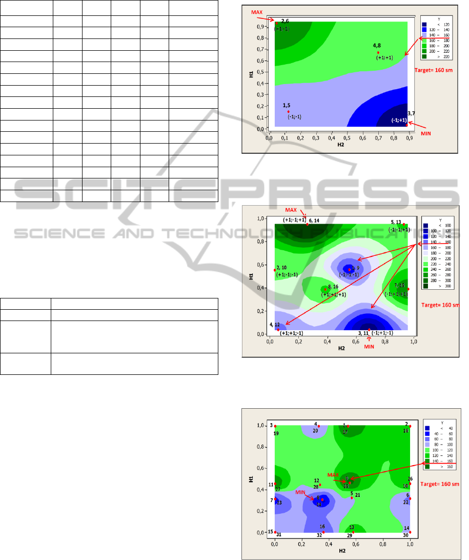
Table 4: Design matrix (experimental plan) for 4 factor
DOE (2 levels 2 replicate experiment).
Run Order X1 X2 X3 X4 MIN/MAX
1, 17 -1 -1 -1 -1
2, 18 +1 -1 -1 -1
3, 19 -1 +1 -1 -1
4, 20 +1 +1 -1 -1
5, 21 -1 -1 +1 -1
6, 22 +1 -1 +1 -1
7, 23 -1 +1 +1 -1
8, 24 +1 +1 +1 -1 MIN
9, 25 -1 -1 -1 +1 MAX
10, 26 +1 -1 -1 +1
11, 27 -1 +1 -1 +1
12, 28 +1 +1 -1 +1
13, 29 -1 -1 +1 +1
14, 30 +1 -1 +1 +1
15, 31 -1 +1 +1 +1
16, 32 +1 +1 +1 +1
Two level factorial designs were analysed by
analysis of variance (ANOVA) and by regression
analysis. The model equations describing the
relationship between response Y and factors X1, X2,
X3 and X4 are represented in Table 5.
Table 5: Model equations for 2, 3 and 4 factor DOE.
DOE type Models equations
2 factor Y= 160.3 + 30,62X1 - 24,75X2 -3X1*X2
3 factor
Y= 212,50 + 28,62X1 - 21,75X2 +
62,25X3 - 19,38X1*X2 - 10,37X1*X3 +
4,75X2*X3 - 13,62X1*X2*X3
4 factor
Y= 105,87 - 15,46X1 - 19,28X2 -
27,69X3 + 14,80X4
The goal of many designed experiments is to
determine the optimal factors settings that produce
the best value for a response of interest. To specify
the goal three options were chosen: Maximize,
Minimize and target distance 160 cm. These three
options were chosen because in industry and science
different goals can be met in solving optimization
problem (MAX, MIN or definite value).
The projection of factors settings (experimental
condition) and response (firing distance values) in
H1/H2 coordinates for 2, 3, 4 factor experiments are
illustrated in Figures 3, 4 and 5, correspondingly.
The experimental running points (corresponding to
the setting parameters) are complemented with
levels (+1;-1) for factors X1 and X2 in the case of 2
factor experiment as well as for factors X1, X2, X3
in the case of 3 factor experiment. In the case of 4
factors experiment the levels of X1-X4 can be found
in Table 4.
The location of MAX, MIN and Target=160 cm are
shown in red colour in Figures 3, 4 and 5.
Figure 3: The projection of factors settings (experimental
condition) and response (firing distance values) in H1/H2
coordinates for 2 factors experiment.
Figure 4: The projection of factors settings (experimental
condition) and response (firing distance values) in H1/H2
coordinates for 3 factors experiment.
Figure 5: The projection of factors settings (experimental
condition) and response (firing distance values) in H1/H2
coordinates for 4 factors experiment.
SIMULTECH2014-4thInternationalConferenceonSimulationandModelingMethodologies,Technologiesand
Applications
764

Table 6: Minitab response optimizer and NN mapping summary results for 2, 3 and 4 factor full factorial DOEs.
Type of
DOE
Goal,
cm
Global solution (FD,
Minitab)
NN map results
(levels of factors in
opt. point)
Run order
(see Tables
2,3,4)
Predicted
Y, cm
Desir-
ability
2 factor
DOE
Max
221
X1=D; X2=1
(+1;-1)
(+1;-1)
(2, 6)
Y=218,5 D=0,978
Min
106
X1=B; X2=3
(-1;+1)
(-1;+1)
(3,7) Y=107,8 D=0,985
Target
=160
X1=B; X2=1
(-1;-1)
NA NA Y=151,3 D=0,838
3 factor
DOE
Max
344
X1=D; X2=1; X3=4A
(+1;-1;+1)
(+1;-1;+1) (6, 14) Y=343 D=0,996
Min
90
X1=B; X2=3; X3=2A
(-1;+1;-1)
(-1;+1;-1) (3, 11) Y=90,5 D=0,998
Target
=160
X1=D; X2=2,93≈3; X3=2A
(+1;+1;-1)
NA NA Y=160 D≈1,0
4 factor
DOE
Max
170,5
X1=B; X2=2A; X3=1;
X4=G
(-1;-1;-1;+1)
(-1;-1;-1;+1)
(9, 25)
Y=170,5 D=1,00
Min
32,2
X1=D; X2=4A; X3=3;
X4=E
(+1;+1; +1;-1)
(+1;+1; +1;-1)
(8, 24)
Y=32,25 D=0,99
Target
=160
X1=B; X2=2A; X3=1,5;
X4=G
≈ (-1;-1;-1+1)
(-1;-1;-1+1)
Close to
(9, 25)
Y=160 D=1,00
Table 6 represents the summary optimization results
including calculations using Minitab response
optimizer for FD as well as NN mapping
visualisation results.
In the case of MAX and MIN values we have got
concordance of results obtained using both methods.
Thus, MAX for global solution as well as for NN
mapping (see Figure 3) in the case of 2 factor DOE
corresponds to setting X1,X2 equal to (+1;-1) and
MIN corresponds to the opposite setting (-1;+1). In
the case of 3 factor DOE we have got MAX at
setting X1,X2,X3 (+1;-1;+1) and MIN at setting (-
1;+1;-1). 4 factor DOE indicates the MAX at setting
(-1;-1;-1;+1) and MIN at setting (+1;+1; +1;-1).
The target equal to 160 cm for 2 factor DOE was
found at the setting X1,X2 (-1;-1) as a global
solution (Minitab calculations) with desirability
0,838. The NN map in Figure 3 shows the line
between blue and green light colours. Additional
calculation should be done for finding the desired
levels for this target which is not in scope of present
article. In the Table 6 it was marked as not available
(NA). For 3 factor DOE Minitab response optimizer
offered the setting X1,X2,X3
(+1;+1;-1) with
desirability 1,0. The NN map in Figure 4 shows the
round lines between blue zone colours marked with
red arrows. Additional calculation should be also
done for finding the desired levels here (not
available (NA) in Table 6). In the case of 4 factor
DOE we have got target close to maximal value in
both methods.
4 CONCLUSIONS
In the paper we demonstrated how different methods
(particularly, factorial designs and neural network
mapping) provide information about optima or
target. No additional experiments are required to
perform both methods. (The same data were used).
The model equations obtained using FD were
replaced by an equivalent NN. The transformation of
multidimensional data into two dimensional maps
enables the full mapping of the objective function
and identification of multiple optima easily. This is
an important feature not presented by conventional
optimization methods like FD or others statistical
methods.
NN mapping technique enables the visualisation
of studied process (response) in 2D map. In some
cases the target can be represented as a region (area).
Engineers can use such areas for determination of
specification limits.
The FFBN NN mapping technique is simple in
use, non- time consuming and can be recommended
for wide use in different industries.
ACatapult.SearchingOptimaUsingFactorialDesignsand2D-NeuralNetworkMappingTechnique-ATutorial
765

ACKNOWLEDGEMENTS
Authors thank the Slovenian Ministry of Higher
Education, Science and Technology (grant P1-017)
and 3ZEN d.o.o. for experimental work.
REFERENCES
Changyu, S., Lixia, W., Qian, L., 2007. Optimization of
injection molding process parameters using
combination of artificial neural network and genetic
algorithm method, J. Mater. Process. Technol.,
vol.183 (2), pp. 412–418.
Cook, D. F., Ragsdale, C. T., Major, R. L., 2000.
Combining a neural network with a genetic algorithm
for process parameter optimization, Eng. Appl. Artif.
Intell., vol. 13, issue 4, pp.391-396.
Daszykowski, M., Walczak, B., Massart, D. L., 2003. A
journey into low-dimensional spaces with
Autoassociative Neural Networks, Talanta, vol. 59 no.
6, pp. 1095-1105.
Daszykowski, M., Walczak, B., Massart, D. L., 2003.
Projection methods in chemistry, Chemom. Intell. Lab.
Syst., vol. 65, pp. 97-112.
Davies, O. L., 1956. Design and Analysis of Industrial
Experiments, Imperial Chemical Industries. London.
Douglas, C. Montgomery, 2012. "Design and Analysis of
Experiments, JOHN WILLEY & SONS, INC.New
York (NY), 8th Edition.
Eriksson, L., Johansson, E., Kettaneh-Wold N., et al.,
2008. Design of Experiments: Principles and
Applications, UMETRICS AB. Sweden, 3-d ed.
Hamdy, M., Hasan, A., Siren, K., 2011. Applying a multi-
objective optimization approach for Design of low-
emission cost-effective dwellings. Build. Environ.,
vol. 46, issue 1, pp.109-123.
Jin, Y., 2011. Surrogate-assisted evolutionary
computation, Recent advances and future challenges.
Swarm and Evolutionary Computation, vol.1(2), pp.
61–70.
Kramer, M. A., 1991. Nonlinear principal component
analysis using autoassociative neural networks, AIChE
J, vol. 37, no. 2, pp. 233–243.
Livingstone, D. J., Hesketh, G., Clayworth, D., 1991.
Novel methods for the display of.
multivariate data using neural networks, J. Mol. Graphics,
vol. 9, pp. 115–118.
Loshchilov, I., Schoenauer, M., Sebag, M., 2010.
Comparison-Based Optimizers Need Comparison-
Based Surrogates. Parallel Problem Solving from
Nature (PPSN XI). Springer, vol. 6238, pp. 364–373.
Natrella, M. G., 1963. Experimental Statistics. National
Bureau of Standards Handbook 91, John Wiley and
Sons. Inc.Washington.
Ozcelik, B., Erzurumlu, T., 2006. Comparison of the
warpage optimization in the plastic injection molding
using ANOVA, neural network model and genetic
algorithm, J. Mater. Process. Technol., vol. 171, issue
3, pp. 437–445.
Park, Y. W., Rhee, S., 2008. Process modeling and
parameter optimization using neural network and
genetic algorithms for aluminum laser welding
automation, The Int. J. Adv. Manuf. Technol., vvol. 37,
issue 9-10, pp. 1014-1021.
Pishvaee, M., Rabbani, M., Torabi, S., 2011. A robust
optimization approach to closed-loop supply chain
network design under uncertainty. Appl. Math.
Modell., vol. 35, issue 2, pp. 637-649.
Sette, S., Boullart, L., et al., 1997. Optimizing the Fiber-
to-Yarn Production Process with a Combined Neural
Network/Genetic Algorithm Approach, Text. Res. J.,
vol. 67 (2), pp. 84-92.
Wu, A., Zhang, J., Chung, H., 2011. Decoupled optimal
design for power electronic circuits with adaptive
migration in coevolutionary environment. Appl. Soft
Comput. J., vol. 11, issue 1, pp. 23-31.
Wang, J., Zhai, Z. J., Jing,Y., et al., 2010. Particle swarm
optimization for redundant building cooling heating
and power system. Appl. Energy, vol. 87, issue 12, pp.
3668-3679.
Zheng, J., Wang, Q., Zhao, P., et al., 2009. Optimization
of high-pressure die-casting process parameters using
artificial neural network, International journal,
advanced manufacturing technology, vol. 44(7-8), pp.
667-674.
SIMULTECH2014-4thInternationalConferenceonSimulationandModelingMethodologies,Technologiesand
Applications
766
