Occupational Diseases Risk Prediction by Cluster Analysis and

Genetic Optimization

Antonio di Noia

, Paolo Montanari

and Antonello Rizzi

Department of Information Engineering, Electronics and Telecommunications, University of Rome "La Sapienza"

Via Eudossiana 18, Rome, Italy

Research Department, National Institute for Insurance against Accidents at Work (INAIL), Rome, Italy

Keywords: Occupational Diseases, Risk Prediction, Computational Intelligence, Cluster Analysis, Genetic Algorithm.

Abstract: This paper faces the health risk prediction problem in workplaces through computational intelligence

techniques applied to a set of data collected from the Italian national system of epidemiological

surveillance. The goal is to create a tool that can be used by occupational physicians in monitoring visits, as

it performs a risk assessment for workers of contracting some particular occupational diseases. The

proposed algorithm, based on a clustering technique is applied to a database containing data on occupational

diseases collected by the Local Health Authority (ASL) as part of the Surveillance National System. A

genetic algorithm is in charge to optimize the classification model. First results are encouraging and suggest

interesting research tasks for further systems’ development.

1 INTRODUCTION

Employee health care is gaining attention by both

private and public companies, as well by OHS

(Occupational Health and Safety) organizations

worldwide. In fact, part of the public costs dedicated

to healthcare can be reduced by monitoring and

controlling workplaces hazards. In this scenario, a

potentially useful challenge is to apply data mining

and knowledge discovery techniques on related

databases, extracting useful information to perform

occupational hazard assessment by health risk

classification methods. To this aim, several studies

show that the application of computational

intelligence techniques can lead to reveal the

existence of structures in the data difficult to detect

with other approaches. For example, in (Chinmoi et

al, 2012) have been developed a decision support

system for employee healthcare, while in (Razan et

al, 2010) have been applied clustering techniques to

medical data to predict the likelihood of diseases. In

(Zhaohui Huang Daoheng Yu Jianye Zhao, 2000)

artificial neural networks have been applied by

Zhaohui Huang Daoheng Yu Jianye Zhao in

occupational diseases incidence forecast.

This work shows the first results of a study for

the application of techniques of data analysis and

computational intelligence to an occupational

diseases database. The goal is the development of a

tool for predicting the likelihood of contracting a

disease as a function of some characteristics of both

the worker and the working environment. The

database contains data collected over a decade by

the Local Health Authority of the Italian Lombardy

region. The problem of identifying possible causes

of risk hazards in work places has been formulated

as a classification one. To this aim, a suited

classification system has been developed, relying on

cluster analysis as the core procedure of the machine

learning engine. In order to automatically determine

both the parameters of the dissimilarity measure

between patterns and to identify the best structural

complexity of the classification model (number of

clusters), a genetic algorithm has been employed to

synthetize the best performing classifier.

2 DATA PROCESSING

The data set has been extracted from the archive of

occupational diseases collected by the Local Health

Authority (ASL) as part of the National System of

Surveillance "MalProf", managed by the National

Institute for Insurance against Accidents at Work

(INAIL). The data set contains records for each

pathology collected from ASL, storing information

Di Noia A., Montanari P. and Rizzi A..

Occupational Diseases Risk Prediction by Cluster Analysis and Genetic Optimization.

DOI: 10.5220/0005077800680075

In Proceedings of the International Conference on Evolutionary Computation Theory and Applications (ECTA-2014), pages 68-75

ISBN: 978-989-758-052-9

 2014 SCITEPRESS (Science and Technology Publications, Lda.)

on registry of the worker, on his work history and

his pathology. For each worker more than one record

may be present in the archive (a single record for

each pathology).

In order to develop and test the whole prediction

system, a first data set with controlled cardinality

has been defined by considering only the cases of

the Lombardy Italian region recorded in the period

1999-2009. Moreover, in order to simplify pattern’s

structure, only records related to workers with a

single pathology and an occupational history

consisting of a single working activity have been

considered. This data set has been cleaned removing

ambiguous situations, inconsistent or missing data.

This first preprocessing step yielded a data set of

3427 records as shown in Table 1; as a further

filtering, the data set records of diseases below the

5% rate were not considered, yielding the final data

set of 2722 records, covering about 80% of cases,

highlighted with colored background in Table 1.

Table 1: Records distribution for pathology.

Disease

. of

records

Cumulative

. of records

Freq.

Cumulative

Freq.

Hearing loss 1493 1493 0.436 0.436

Spinal diseases 334 1827 0.097 0.533

musculoskeletal

disorders

(excluding

spinal diseases)

288 2115 0.084 0.617

Tumors of the

pleura and

peritoneum

232 2347 0.068 0.685

Carpal tunnel

syndrome

199 2546 0.058 0.743

Skin diseases 176 2722 0.051 0.794

Disorders of the

ear (except

hearing loss)

137 2859 0.040 0.834

Mental illness 98 2957 0.029 0.863

Diseases of the

respiratory

system

76 3033 0.022 0.885

Other diseases 394 3427 0.115 1

The final available data set has been partitioned

into three subsets by random stratification: the

training set (50% of the total number of available

patterns, denoted with S

), the validation set (25%,

VAL

) and the test set (the remaining 25%, S

TEST

Table 2 shows the distribution of diseases and their

labels as integer numbers codes. The similarity

between the subjects was evaluated through a

distance function based on 6 features (Table 3), both

numerical and categorical, identified by a

preliminary analysis of data and knowledge in the

field.

Table 2: Pathologies in descending order of frequency.

Pathologies Training set

Validation set

1 - Hearing loss

747

54.89%

373

54.85%

2 - Spinal diseases

167

12.27%

12.21%

3 - Musculoskeletal

disorders

144

10.58%

10.59%

4 - Tumors of the pleura

and peritoneum

116

8.52%

8.53%

5 - Carpal tunnel

7.27%

7.35%

6 - Skin diseases

6.47%

Total

1361

100%

680

100%

Table 3: Features.

Code Meaning Data Type

Age of the worker at the time

of disease assessment (years)

numerical

Duration of the working

period (months)

numerical

Age at the beginning of the

working period (years)

numerical

x4 Gender categorical

Profession carried out by the

worker

categorical

x6 Company's economic activity categorical

The profession of the worker is coded through a

pair of characters based on the Italian version of the

classification system ISCO. The International

Standard Classification of Occupations (ISCO) is a

tool for organizing jobs into a clearly defined set of

groups according to the tasks and duties undertaken

in the job. The economic activity of the company is

coded by a pair of characters based on the Italian

version of the NACE classification system. NACE

(Nomenclature des Activités Économiques dans la

Communauté Européenne) is a European industry

standard classification system similar in function to

Standard Industry Classification (SIC) and North

American Industry Classification System (NAICS)

for classifying business activities.

3 THE PROPOSED ALGORITHM

In order to design an algorithm able to evaluate the

probability of contracting an occupational disease as

OccupationalDiseasesRiskPredictionbyClusterAnalysisandGeneticOptimization

a function of some characteristic of the worker, his

work history and his work environment, the risk

prediction problem has been reformulated as a

classification problem. The basic classification

system is a clustering based one, which is trained in

a supervised fashion, by discovering clusters of

labelled patterns in S

. Once the clusters are

identified, the classification rule is defined by

considering, within each cluster, the class label with

higher frequency. A test pattern is classified by

assigning the class label according to the cluster

representative label having minimum dissimilarity

value. The algorithm was coded in C++ language.

3.1 Basic Algorithm

The core procedure during the synthesis of a

classification model consists in clustering S

by the

well –known k-means algorithm. To this aim, an ad

hoc dissimilarity measure δ between patterns was

defined as a convex linear combination of inner

dissimilarity measures δ

between homologues

features:







vupvu

,),(



(1)

where N is the number of the features (6 in our case)

and



1,0; 

is the relative weight of the i-

th feature.

The δ

(u,v) distance between patterns u and v

relative to the i-th feature have been defined

differently on the basis of the considered feature

type, which can be continuous or categorical

(discrete nominal) values:

 for age (in years) and the duration of the activity

(in months), δ

is the Euclidean distance

normalized in the unitary interval [0,1];

 for gender and economic activity of the

company, in the case of concordance δ

= 0,

otherwise δ

= 1 (simple match);

 for the job of the individual, in the case of

concordance of both characters δ

= 0, in the case

of concordance of the first character only δ

= ½,

otherwise δ

= 1.

The overall classification system has been

designed to automatically determine the weights p

of the dissimilarity measure (1) and the optimal

number of clusters k, in order to maximize the

classification accuracy:







Kxx

accuracyf ),(



(2)

where:

S is the labelled pattern set on which is computed the

accuracy;

Ω = {hearing loss, spinal diseases, musculoskeletal

disorders, tumors of the pleura and peritoneum,

carpal tunnel syndrome, skin diseases} is the

considered label set;







is the pathology of worker

Sx 

(ground

true class label);







is the label assigned by the classification

model to x;

h(ω

, ω

) = 1 if ω

= ω

;

h(ω

, ω

) = 0 if ω

≠ ω

;

In order to perform this optimization task, we

have developed a suited implementation of a genetic

algorithm. The generic individual of the population

subject to evolution by genetic operators is formed

of two data structures (sections) for a total of 7

parameters to be optimized:

1. a vector of 6 real numbers between 0 and 1,

corresponding to the weights associated with

the features in the distance function δ;

2. an integer between 2 and a maximum value

fixed in the system parameters, corresponding

to the number of clusters to be used for the

clustering of the training set.

From one generation to the next, each individual

in the GA is evaluated by a fitness function defined

as the accuracy (2), computed on S

VAL

. The selection

is simulated using a roulette wheel operator. The

crossover and mutation affect the entire individual,

formed by six weights and the number of clusters.

The individuals of the initial population of the

GA are created as random samples. For each

individual, a clustering procedure with k-means is

performed on the training set with weights fixed in

the first section of the individual’s genetic code and

setting the number of clusters as the integer number

stored in the second section. Once obtained a

partition of the S

, each cluster is assigned with a

unique label, defined as the most frequent pathology

in the cluster. Successively the fitness is computed

as the classification accuracy on the validation set,

according to (2).

Reproduction, crossover and mutation are

applied to the individuals of the GA to evolve the

population, until a stop criterion based on a

maximum number of generations is met. The

algorithm is summarized in Table 4.

The distribution of pathologies in the data set

shows that class labels (diseases) are not well

balanced, and this could distort the values of fitness

by giving excessive importance to the most frequent

pathology. Therefore, it is introduced a variant of

ECTA2014-InternationalConferenceonEvolutionaryComputationTheoryandApplications

fitness function aiming to equally weight all

misclassifications, regardless of their number. The

new fitness (equation (3)) is given by the weighted

accuracy, i.e. the mean value of the percentages of

correct answers for each pathology. Tests were

performed with both fitness and the results have

been compared.













Kxxweighted

accuracyf ),(

(3)

where:

is the subset of S of all elements associated with

pathology





(

SS 



Table 4: Summary of the basic algorithm.

Input parameters:

- Maximum number of clusters: Kmax

- Number of population’s individuals in the GA: Pop

- Number of generations of GA: nGeneration.

1. Reading data from S

and S

VAL.

2. Initialization (Generation = 0).

For j = 1 to Pop

o Random assignment of weights p

of the 6

features and of the value K ≤ Kmax.

o Clustering of the elements of S

into K

clusters using the distance function (equation 3)

with the parameters encoded in the individual j

o Evaluation of the fitness of individual j with

the function

in equation 1

3. For q = 1 to nGeneration

o Application of elitism.

o Repeat



Selection of individuals of the old population

by roulette wheel operator.

 Crossover between pairs of the selected

individuals.

 Mutation with a low probability on each

element.



Clustering of S

in K clusters using the

distance function (1) with the parameters

encoded in the individual.



Evaluation of the fitness function (2) on S

VAL

Until complete new generation

3.2 A Second Variant of the Algorithm

The basic algorithm leads to the formation of

clusters containing more than one disease. The label

associated with the cluster coincides with the most

frequent pathology in it. This procedure cannot

assure the presence of at least one cluster for each

class. To make sure that all the pathologies are

represented in the final classification model, a

second version of the proposed classification system

has been designed.

For this purpose, the training set S

has been

partitioned into six subsets, one for pathology. The

new algorithm runs six cluster analyses in parallel,

one for each of the 6 subsets of S

. As a

consequence, each cluster will contain patterns

associated with a unique class label and will

consequently be directly labeled. The union of the

six sets of labeled clusters originated will be directly

employed for the classification model definition.

The generic individual of the population of the

GA has been adapted to the new algorithm; in

particular, the second part of the individual no

longer contains a single integer, but 6 integers, each

representing the number of clusters to use in the 6

cluster analysis performed in parallel on each subset

of the training set (one for each class label). The

initialization step of the first generation of the GA is

similar to the basic algorithm. As for the previous

version, we considered both the fitness functions f

and f

computed on S

VAL

(Equations (2) and (3)) for

individual fitness evaluation.

4 RESULTS

All experiments were conducted using the GA by

evolving a population of 100 individuals for 50

generations, fixing to 20 the maximum number of

clusters. All performances reported in the following

tables are computed on the test set. Table 5 shows

the classification results as a confusion matrix, in the

case of the basic algorithm and using equation (2) as

fitness. All correct guesses are located in the

diagonal (highlighted in gray) of the table, so it is

easy to inspect visually the table for errors, as they

will be represented by any non-zero value outside

the main diagonal.

For each of the 6 diseases, further views can be

extracted from the Confusion matrix in the

Confusion table’s schema (see Table 6). Given the

content of the dataset, formed only by workers

affected by pathologies, for each disease are

considered as healthy the workers not affected from

that pathology. The columns “Positive to test” and

“Negative to test” of Confusion tables contain the

number of workers that the algorithm predicts

respectively as sick (i.e. affected by the disease in

question) or healthy (i.e. affected by other diseases).

The rows “Actual true” and “Actual false” contain

the number of those who actually are, respectively,

sick and healthy. For example, the two confusion

tables (table 7a and 7b) shown below summarize the

cases “1-hearing loss” and “4-

tumours of the pleura

and peritoneum”.

OccupationalDiseasesRiskPredictionbyClusterAnalysisandGeneticOptimization

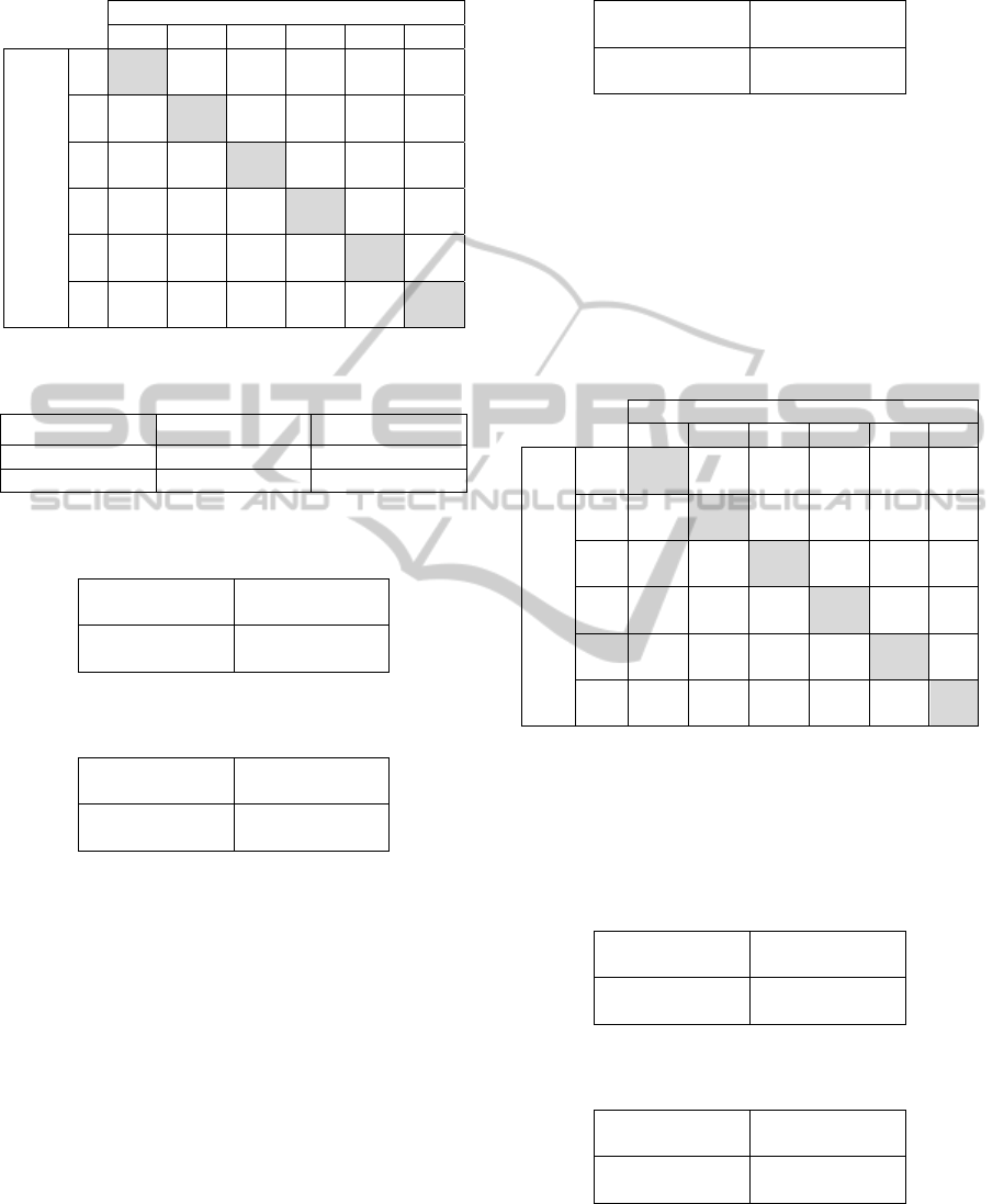
Table 5: Confusion matrix for basic algorithm with f

. In

brackets normalized values as percentage.

Predicted class

1 2 3 4 5 6

Actual

class

351

(94.1)

(1.3)

(0.0)

(1.9)

(2.4)

(0.3)

(54.2)

(43.4)

(0.0)

(1.2)

(44.4)

(27.8)

(0.0)

(22.2)

(5.6)

(31.0)

(13.8)

(0.0)

(55.2)

(0.0)

(18.0)

(32.0)

(0.0)

(2.0)

(46.0)

(2.0)

(45.5)

(15.9)

(0.0)

(9.1)

(29.5)

Table 6: Confusion table’s schema for the evaluation of

the predictive ability of a test.

Positive to test Negative to test

Actual true True positives False negatives

Actual false False positives True negatives

Table 7a: Confusion table for pathology “1-hearing loss” –

basic algorithm using f

351

True positives

False negatives

124

False positives

183

True negatives

Table 7b: Confusion table for pathology “4- tumors of the

pleura and peritoneum” – basic algorithm using f

True positives

False negatives

False positives

614

True negatives

The confusion tables allow more detailed

analysis than mere proportion of correct guesses

(accuracy). Accuracy is not a reliable metric for the

real performance of a classifier, because it will yield

misleading results if the data set is unbalanced. For

example, if there were 95 sick and only 5 healthy in

the data set, the classifier could easily be biased into

classifying all the samples as sick. The overall

accuracy would be 95%, but in practice the classifier

would have a 100% recognition rate for the sick

class and a 0% recognition rate for the wealthy class.

For these reasons, we reported the overall confusion

table (see table 8) containing the average values for

all classes.

Table 8: Confusion table with average values - basic

algorithm with f

75.8

True positives

37.5

False negatives

37.5

False positives

529.2

True negatives

The results of the second experiment, based on

the basic algorithm using the fitness f

, are shown in

table 9. The number of clusters of the best individual

of the last generation is 20, of which 13 are labeled

as "1 - hearing loss, 2 as "2 - spinal diseases", 1 as

"3 - musculoskeletal disorders", 2 as " 4 - tumors of

the pleura and peritoneum", 1 as "5 - carpal tunnel"

and 1 as " 6 - skin diseases."

Table 9: Confusion matrix for basic algorithm with f

. In

brackets normalized values as percentage.

Predicted class

1 2 3 4 5 6

Actual

class

338

(90.6)

(1.9)

(4.0)

(1.6)

(0.0)

(43.4)

(42.2)

(4.8)

(0.0)

(8.4)

(1.2)

(44.4)

(16.7)

(19.4)

(0.0)

(18.1)

(1.4)

(31.0)

(1.7)

(12.1)

(55.2)

(0.0)

(16.0)

(12.0)

(24.0)

(4.0)

(42.0)

(2.0)

(47.7)

(6.8)

(0.0)

(18.2)

(27.3)

Similarly to the previous case, the two confusion

tables (table 10a and 10b) summarize the cases “1 –

hearing loss” and “4 – tumours of the pleura and

peritoneum”.

Table 10a: Confusion table for pathology “1 – hearing

loss” – basic algorithm using f

338

True positives

False negatives

115

False positives

192

True negatives

Table 10b: Confusion table for pathology “4 – tumors of

the pleura and peritoneum” – basic algorithm using f

True positives

False negatives

False positives

605

True negatives

The final confusion table containing the average

values for all classes concerning the second

experiment is shown in Table 11.

ECTA2014-InternationalConferenceonEvolutionaryComputationTheoryandApplications

Table 11: Confusion table with average values - basic

algorithm with f

75.3

True positives

38.0

False negatives

38.0

False positives

528.7

True negatives

In the third experiment, based on the proposed

variant of the algorithm using the fitness f

, the best

individual of the last generation shows an overall

classification accuracy equal to 62%. The total

number of clusters was 36, with the following class

distribution: 20 are labelled as "1 - hearing loss", 6

as "2 – spinal diseases," 2 as "3 - musculoskeletal

disorders", 4 as "4 - tumors of the pleura and

peritoneum", 2 as "5 - carpal tunnel" and 2 as "6 -

diseases of the skin". In table 12 are summarized the

data of the six tables of confusion (one for disease).

Each column represents the confusion table for the

indicated disease in the column header. The final

table of confusion with average values is shown in

Table 13.

Table 12: Summarized data of the confusion tables -

variant of the algorithm with f

Pathology

1 2 3 4 5 6

True

positives

312 42 12 35 1 19

False

positives

127 59 19 15 20 19

False

negatives

61 41 60 23 49 25

True

negatives

180 538 589 607 610 617

Table 13: Confusion table with average values – variant of

the algorithm with f

70.2

True positives

43.2

False negatives

43.2

False positives

523.5

True negatives

In the fourth experiment, based on the variant of

the algorithm with the fitness f

, we obtained the

53% of correct classification in correspondence of

the best individual of the last generation. The total

number of clusters was 71, with the following class

distribution: 18 are labeled as "1 - hearing loss", 10

as "2 - spinal diseases", 7 as "3 - musculoskeletal

disorders", 11 as "4 - tumors of the pleura and

peritoneum", 15 as "5 - carpal tunnel", 10 as "6 -

skin diseases". The results for this experiment are

shown in Table 14 and in Table 15

Table 14: Summarized performances of the confusion

tables - variant of the algorithm with f

Pathology

1 2 3 4 5 6

True

positives

210 44 17 35 30 25

False

positives

48 61 45 30 89 46

False

negatives

163 39 55 23 20 19

True

negatives

259 536 563 592 541 590

Table 15: Confusion table with average values – variant of

the algorithm with f

60.2

True positives

53.2

False negatives

53.2

False positives

513.5

True negatives

Table 16: Chromosome of GAs.

Basic

Algorithm

using f

Basic

Algorithm

using f

Variant of

Algorithm

using f

Variant of

Algorithm

using f

Feature x1 1.000 1.000 0.870 0.660

Feature x2 0.041 0.134 0.894 0.709

Feature x3 0.078 0.346 0.569 1.000

Feature x4 0.592 0.519 1.000 0.196

Feature x5 0.189 0.220 0.280 0.726

Feature x6 0.265 0.076 0.096 0.141

N. cluster 10 20 – –

N. cluster

pathology 1

– – 20 18

N. cluster

pathology 2

– – 6 10

N. cluster

pathology 3

– – 2 7

N. cluster

pathology 4

– – 4 11

N. cluster

pathology 5

– – 2 15

N. cluster

pathology 6

– – 2 10

The Table 16 shows the genetic code of the best

individual produced by the GA for each experiment.

The first six parameters encode the weight of the

features (normalized values) and the other

parameters encode the clusters num

ber.

Another significant tool for performance

analysis, commonly used in the evaluation of

diagnostic tests, consists in the use of sensitivity and

specificity. Let us consider a study evaluating a new

test that screens people for a disease. The test

outcome can be positive (predicting that the person

is affected by the considered disease) or negative

OccupationalDiseasesRiskPredictionbyClusterAnalysisandGeneticOptimization

(predicting that the person is healthy). The test

results for each subject may or may not match the

subject's actual status. In that setting:

 True positive: Sick people correctly

diagnosed as sick

 False positive: Healthy people incorrectly

identified as sick

 True negative: Healthy people correctly

identified as healthy

 False negative: Sick people incorrectly

identified as healthy

The four outcomes can be expressed in a 2×2

confusion table, as in Table 17a. In table 17b are

defined the indicators used in diagnostic tests.

Table 17a: Confusion table.

Condition

positive

Condition

negative

Test

positive

True

positive

False

positive

Test

negative

False

negative

True

negative

Table 17b: Diagnostic Tests indicators.

Sensitivity = True positive / Σ Condition positive

Specificity = True negative / Σ Condition negative

Positive predictive value = True positive / Σ Test positive

egative predictive value = True negative / Σ Test neg.

In Table 18 are briefly described the diagnostic

test's indicators, using the average values calculated

on all pathologies. Table 19 summarizes the results

of 11 runs, with different initial seeds for the random

number generator, using the variant of algorithm

with f

. For both negative and positive predictive

values are reported the average performance,

standard deviation, minimum and maximum values,

for each disease and for the totality of the

pathologies.

Table 18: Diagnostic test’s indicators – average values.

Basic

Algorithm

using f

Basic

Algorithm

using f

Variant of

Algorithm

using f

Variant of

Algorithm

using f

Sensitivity 0.447 0.461 0.427 0.517

Specificity 0.905 0.907 0.895 0.901

Negative

predictive

value

0.929 0.923 0.906 0.892

Positive

predictive

value

0.503 0.574 0.460 0.442

Table 19: Negative and positive predictive values by

pathology resulting from a pool of 11 runs (variant of

Algorithm using f

Pathology 1 2 3 4 5 6 All

Patterns 373 83 72 58 50 44 680

Negative

predictive

value

Average 0,58 0,94 0,90 0,97 0,97 0,97 0,90

St. dev. 0,02 0,01 0,01 0,01 0,01 0,00 0,01

Min 0,54 0,92 0,90 0,96 0,96 0,96 0,89

Max 0,61 0,94 0,91 0,98 0,98 0,98 0,91

Positive

predictive

value

Average 0,82 0,38 0,26 0,48 0,28 0,28 0,50

St. dev. 0,01 0,03 0,05 0,09 0,03 0,04 0,03

Min 0,81 0,34 0,21 0,40 0,22 0,23 0,44

Max 0,85 0,43 0,35 0,67 0,34 0,35 0,53

In Tables 20 and 21 are shown the diagnostic

test’s indicators relative, respectively, to the

"hearing loss" and to the "tumors of the pleura and

peritoneum".

Table 20: Indicators relative to “1 – hearing loss”.

Basic

Algorithm

using f

Basic

Algorithm

using f

Variant of

Algorithm

using f

Variant of

Algorithm

using f

Sensitivity 0.941 0.906 0.836 0.563

Specificity 0.596 0.625 0.586 0.844

Negative

predictive

value

0.893 0.846 0.747 0.614

Positive

predictive

value

0.739 0.746 0.711 0.814

Table 21: Indicators relative to “4 - tumors of the pleura

and peritoneum”.

Basic

Algorithm

using f

Basic

Algorithm

using f

Variant of

Algorithm

using f

Variant of

Algorithm

using f

Sensitivity 0.552 0.552 0.603 0.603

Specificity 0.987 0.973 0.976 0.952

Negative

predictive

value

0.959 0.959 0.963 0.963

Positive

predictive

value

0.800 0.653 0.700 0.538

ECTA2014-InternationalConferenceonEvolutionaryComputationTheoryandApplications

5 CONCLUSIONS

The first experiment (basic algorithm using f

)

shows that the sensitivity has a very high value

(0.941) for the group “hearing losses” (larger group),

and an average value equal to 0.447. The pathology

“3 - musculoskeletal disorders” was never predicted

by the algorithm. The specificity presents a value

close to 0.6 for the group “hearing loss” and an

average value greater than 0.9. These first results

show that function f

privileges the most frequent

pathology. In the second experiment (basic

algorithm using f

), the sensitivity no longer has null

values. The average sensitivity is equal to 0.461,

value slightly better than the previous case. The

specificity has values similar to the ones in the

previous experiment. The third experiment (variant

of the basic algorithm using f

) shows performance

values in general slightly worse compared to the

basic algorithm. However, there is an improvement

for the sensitivity of some pathologies. The fourth

experiment (variant of the basic algorithm using f

)

shows that the use of f

compared to f

has led to an

improvement of the average sensitivity of almost a

decimal point. Regarding the specificity, for all

pathologies the values are always greater than 0.84,

with an average value of 0.901.

The comparison of the average values of the

indicators (Table 18) shows how the second

algorithm with f

present the highest sensitivity.

Regarding the specificity and the predictive value of

the negative outcome of the test, we have

substantially similar behaviours for the four

experiments. As concerns positive predictive value,

the basic algorithm with f

has provided the best

results. The high values, close to unity, for

specificity and negative predictive value are

encouraging. However, the variant of the algorithm,

while not showing results appreciably better than the

basic algorithm, has better performance by reducing

the execution time to a third compared to the basic

version, because clustering procedures are run on

smaller sets. Thus, for the final commitment of the

system, which has to deal with a much larger

database, the second version should be preferred,

considering also that its performances are very close

to the ones obtained with the basic algorithm. In

particular, as shown by standard deviations in table

19, performances are stable over multiple runs,

assuring a good reliability to the results. Moreover,

the negative predictive value can be considered

sufficient to be used in a suited automatic screening

procedure, designed to reduce costs in performing

clinical trials on all the interested workers, since a

negative classification for a given worker is

sufficient to reliably ascertain his health status. Note

that in general for the groups “hearing loss” (the

largest group) and “tumors of the pleura and

peritoneum” (more severe disease) the results are

better than for other diseases, including the

sensitivity and the positive predictive value.

The examination of the weights of the features

(Table 16) shows different values for the different

algorithms. In all the experiments, only the

economic activity of the company seems less

important than the other features, so it might be

interesting to define a different set of features,

replacing the economic activity.

REFERENCES

A. K. Jane, R. C. Dubes, 1988. Algorithms for Clustering

Data, Prentice-Hall. Englewood Cliffs.

Alexandr A. Savinov, 1999. Mining Possibilistic Set-

Valued Rules by Generating Prime Disjunctions. In

PKDD'99, 3rd European Conference on Principles

and Practice of Knowledge Discovery in Databases.

Vol. 1704 Springer (1999), p. 536-541.

Chinmoy Mukherjee, Komal Gupta, Rajarathnam

Nallusamy, 2012. A Decision Support System for

Employee Healthcare. In Third International

Conference on Services in Emerging Markets.

Kumara Sastry, David Goldberg, Graham Kendall, 2005.

Genetic Algorithms. In Search Methodologies,

Springer US.

Razan Paul, Abu Sayed Md. Latiful Hoque, 2010.

Clustering Medical Data to Predict the Likelihood of

Diseases, IEEE - Digital Information Management

(ICDIM), Fifth International Conference.

Zhaohui Huang Daoheng Yu Jianye Zhao, 2000.

Application of Neural Networks with Linear and

Nonlinear Weights in Occupational Disease Incidence

forecast. In Circuits and systems. IEEE APCCAS

2000.

OccupationalDiseasesRiskPredictionbyClusterAnalysisandGeneticOptimization