
Prediction Model Adaptation Thanks to Control Chart Monitoring
Application to Pollutants Prediction
Philippe Thomas, William Derigent and Marie-Christine Suhner
Université de Lorraine, CRAN, UMR 7039, Campus Sciences, BP 70239, 54506 Vandœuvre-lès-Nancy cedex, France
CNRS, CRAN, UMR7039, 54506 Vandœuvre-lès-Nancy cedex, France
Keywords: Indoor Air Quality, Neural Networks, Relearning, Control Charts.
Abstract: Indoor air quality is a major determinant of personal exposure to pollutants in today’s world since people
spend much of their time in numerous different indoor environments. The Anaximen company develops a
smart and connected object named Alima, which can measure every minute several physical parameters:
temperature, humidity, concentrations of COV, CO
2
, formaldehyde and particulate matter (pm). Beyond the
measurement aspect, Alima presents some data analysis feature named ‘predictive analytics’, whose
primary aim is to predict the evolution of indoor pollutants in time. In this article, the neural network (NN)
model, embedded in this object and designed for pollutant prediction, is presented. In addition with this NN
model, this article also details an approach where batch learning is performed periodically when a too
important drift between the model and the system is detected. This approach is based on control charts.
1 INTRODUCTION
Air pollution is now identified as a major
international issue. However, in people’s mind, it
always refers to the quality of outdoor air, whereas
the predominant environment in this regard is the
residence. Indeed, indoor air quality is a major
determinant of personal exposure to pollutants in
today’s world since people spend much of their time
in numerous different indoor environments (Walsh
et al. 1987).
During the last two decades there has been
increasing concern within the scientific community
over the effects of indoor air quality on health.
Changes in building design devised to improve
energy efficiency have meant that modern homes
and offices are frequently more airtight than older
structures. Furthermore, advances in construction
technology have caused a much greater use of
synthetic building materials, which provide indoor
pollution (Jones 1999).
The known health impacts and corresponding
pollutants are numerous. Table 1 is an excerpt taken
from (Spengler and Sexton, 1983) to illustrate some
of the major indoor pollutants. The sources of
pollution can be located indoor (building material,
furniture, stoves…) or outdoor (air coming through
an opened window or via the ventilation system).
Table 1: Pollutants and sources.
Pollutant Major emission sources
Allergens House dust, domestic animals,
Asbestos Fire retardant materials, insulation
Carbon dioxide Metabolic activity, combustion activities,
Carbon monoxide Fuel burning, boilers, stoves, gas…
Formaldehyde Particleboard, insulation, furnishings
Micro-organisms People, animals, plants, air conditioning
Nitrogen dioxide Outdoor air, fuel burning, motor vehicles
Organic substances Adhesives, solvents, building materials,
Ozone Photochemical reactions
Particles Tobacco smoke, combustion products...
Polycyclic aromatic
hydrocarbons
Fuel combustion, tobacco smoke
Pollens Outdoor air, trees, grass, weeds, plants
Radon Soil, building construction materials
(concrete, stone)
Fungal spores Soil, plants, foodstuffs, internal surfaces
Sulfur dioxide Outdoor air, fuel combustion
Symptoms and consequences of exposure to a
pollutant can vary depending on the pollutant type
and concentration. For example, the carbon dioxide
(whose indoor concentrations can vary from 700 to
3000 ppm) is a simple suffocating gas and can also
act as a respiratory irritant (Maroni et al. 1995),
whereas the exposition to a formaldehyde
concentration of 100 ppm can cause death.
It thus explains why indoor air quality recently
receives much public attention, and people are now
eager to measure in their own homes the quality of
their indoor air. To answer to this growing need, The
Anaximen Company develops a smart and
172
Thomas P., Derigent W. and Suhner M..
Prediction Model Adaptation Thanks to Control Chart Monitoring - Application to Pollutants Prediction.
DOI: 10.5220/0005075501720179
In Proceedings of the International Conference on Neural Computation Theory and Applications (NCTA-2014), pages 172-179
ISBN: 978-989-758-054-3
Copyright
c
2014 SCITEPRESS (Science and Technology Publications, Lda.)

connected object named Alima (Alima, 2013).
In fact, pollutant levels are constantly changing,
depending on the tenants’ activities. Alima can
measure every minute several physical parameters:
temperature, humidity, concentrations of COV, CO
2
,
formaldehyde and particulate matter (pm). Data are
stored on the object or can be sent to a distant
database, and are available for the user online via
phone apps or websites. Beyond the measurement
aspect, the society currently plans to embed in Alima
some data analysis feature named ‘predictive
analytics’, whose primary aim is to predict the
evolution of indoor pollutants in time. Anaximen
and the CRAN laboratory are associated to develop
this leading-edge feature.
In this article, a neural network (NN) model
designed for pollutant prediction is presented.
However, a drift can appear between the NN model
and the system modelled (due to, for example, a
modification of the occupant behavior), and forces
the NN to do a relearning phase. But this relearning
phase is time and resource consuming and should be
done sparingly. So, in addition with the NN model
for pollutant detection, this article also details an
approach where batch learning is performed
periodically when a too important drift between the
model and the system is detected. This approach is
based on control charts.
Section 2 presents a short state-of-the-art on neural
network modelling, section 3 details the approach
used to control the drift and perform the batch
learning while section 4 presents the industrial
application. Section 5 first exposes the results
obtained by the NN model for pollutant prediction
(without any relearning phase), and then describes
the results obtained when using the drift detection
algorithm.
2 NEURAL NETWORK MODEL
Artificial neural network models have been
successfully applied to solve many different
problems, including dynamic systems identification,
patterns classification, adaptive control, functions
approximation and so on.
Among these artificial neural network models, the
multilayer perceptron (MLP) is, by far, the most
popular architecture due to its structural flexibility,
good representational capabilities, and the
availability of a large number of training algorithms
(Han and Qiao 2013). This model is used for both
classification and regression tasks.
Works of Cybenko (1989) and Funahashi (1989)
have proved that a MLP with only one hidden layer
using a sigmoïdal activation function and an output
layer can approximate all non-linear functions with
the wanted accuracy. Its structure is given by:
0
1
2101
21
11
..
n
n
iihhi
ih
zg wg wx b b
(1)
Where:
-
0
h
x
are the n
0
inputs of the neural network,
-
1
ih
w
are the weights connecting the input layer
to the hidden layer,
-
1
i
b are the biases of the hidden neurons,
-
g
1
(.) is the activation function of the hidden
neurons (namely the hyperbolic tangent),
-
2
i
w are the weights connecting the hidden
neurons to the output one,
-
b is the bias of the output neuron,
- g
2
(.) is the activation function of the output
neuron and,
-
z is the network output.
Because the problem is a regression problem, g
2
(.) is
chosen linear.
Three steps must be performed in order to design the
neural model:
initialization, learning and pruning.
The first one is the determination of the initial set of
weights and biases. This step is important because
learning algorithm performs a local search of the
minimum. So, in order to avoid local minimum
trapping, different initial sets must be constructed
which allow beginning to learn in different zones of
the criteria domain. Different initialization
algorithms have been proposed in the literature
(Thomas and Bloch 1997). The initialization
algorithm used in this paper is the one proposed by
Nguyen and Widrow (1990) which allows
associating a random initialization of weights and
biases to an optimal placement in input and output
spaces.
The second step is performed by the learning
algorithm which must fit the network output with the
data. In industrial applications, data are noisy and
corrupted with many outliers. In order to limit the
impact of outliers on the results, a robust Levenberg-
Marquardt algorithm is used (Thomas
et al. 1999).
Levenberg–Marquard algorithm allows associating
the speed of the Hessian methods to the stability of
the gradient methods. This is performed by adding a
parameter multiplied by the identity matrix in order
to permit the inversion of the Hessian matrix even if
it is singular. The tuning of this parameter during the
learning allows the Levenberg–Marquard algorithm
to work as a gradient descent algorithm when this
PredictionModelAdaptationThankstoControlChartMonitoring-ApplicationtoPollutantsPrediction
173

parameter is large and as a Gauss–Newton algorithm
when this parameter is small. The use of a robust
criterion allows to avoid the influence of outliers and
provides a regularization effect in order to prevent
overfitting. An important issue in neural network
design is the determination of its structure. To
determine it, two approaches can be used. The first
one is constructive, where the hidden neurons are
added one after the other (Ma and Khorasani 2004).
The second approach exploits a structure with too
many initial hidden neurons, and then prunes the
least significant ones (Setiono and Leow 2000,
Engelbrecht 2001). We focus on the pruning
approach that allows a simultaneous selection of the
input neurons and the number of hidden neurons.
The pruning phase is performed in two steps. First,
the Engelbrecht algorithm is used which allows to
quickly simplify the structure and second, the
Setiono and Leow algorithm is used which is slower
but also more efficient (Thomas
et al. 2013).
3 ONLINE ADAPTATION OF THE
MODEL
3.1 Generalities
Ideally, the data collected during the
experimentation phase should describe all the states
of the system to model. However, it is sometimes
not feasible due to the high number of potential
situations the system could encounter. Indeed, in our
case data collected are different depending on the
seasons, the yearly weather, changes in user’s habits
and so on. Technically, it would thus be highly
difficult to obtain an exhaustive data set. As a result,
our approach consists in two phases: first, a learning
phase is achieved based on a data set obtained via a
relatively short experimentation phase (in our case, 1
month, see section 4.1) to construct a first “specific”
NN model. Then, a relearning is launched if and
only if a significant difference (called “drift”)
between the system behavior and its corresponding
NN model is detected.
In many case, a drift may appear between the model
constructed and the system studied. This drift may
be due to two main reasons. The first one concerns
the evolution of input parameters. With a learning
approach, the obtained model is valid only on the
learned domain. The model is able to provide a valid
solution only in this concerned domain.
The second reason concerns the uncontrolled
modification of the machine or environment
behavior. Indeed, A change of a parameter
(voluntarily or not, measured or not) which is not an
input of the model, can affect the behavior of the
machine. In this case, this parameter should be part
of the model inputs but, as it was considered
constant for the duration of the learning step, it was
not retained as such. Due to this change, which may
even be unknown to operators and users, the model
will therefore provide results out of step with reality.
To take into account these problems, a relearning
on new data is needed. There are two practical ways
to implement learning in neural networks: batch
training and on-line training. Whenever a new data
is received, batch learning uses this new data
together with the past data to perform a retraining.
But this approach is time consuming. The on-line
approach uses only new data to adapt the model.
However, this approach suffers from slow training
error convergence as a large number of training data
may be required (Liang
et al. 2006). Moreover,
different works have shown that on-line training
strategy does not converge to the optimal weights
(Heskes and Wiegerinck 1996, Nakama 2009).
We thus propose here another approach where a
batch learning is performed periodically when a drift
between the model and the system occurs, in order
to synchronize the model with the reality.
Because this synchronization is time consuming, the
synchronization frequency must be optimized.
Rather than consider a resynchronization frequency
in response to events (arrival of new information
from one of the connected devices, solicitation by an
operator…) or a periodically one (every hour,
week…), it is better to rely on statistical findings.
Among the 7 basic tools for quality control, control
charts, also known as Shewhart charts or process-
behavior charts (Shewhart 1931), are interesting
Statistical Process Control (SPC) tools useful for our
proposed system.
3.2 Control Charts
Control charts are particularly relevant to the
dynamic quality control with the use of time-series
(Tague 2004). They can determine statistically if a
variation is no longer under control. Indeed, it is
known that even when a process is under control
there is approximately a 0.27% probability of a point
exceeding a 3σ control limit (Pareto). These few
isolated points should not trigger synchronization.
But the detection of too many points above this limit
may underlines the presence of a special cause, even
if it is not yet known.
The Combination of a neural network with the
NCTA2014-InternationalConferenceonNeuralComputationTheoryandApplications
174

control charts can therefore inherit from the
robustness of the statistical analysis and the
adaptability of the neural network. Du
et al. (2012)
work on the inverse combination of both tools with a
recognition algorithm of control charts using neural
networks to get alerts in case of quality problems
and to provide clues in defining causes.
In our case, when a set of
n new data is collected,
a performance indicator is calculated and compared
to two bounds determined on the initial validation
data set. If this indicator is still between the two
bounds, the model is always suitable. If the new
value of the indicator is outside the bounds, a
relearning phase is needed on these new collected
data. Figure 1 shows an example of control chart to
monitor the accuracy of the model. It presents the
evolution of the considered indicator compared to
the upper (UCL) and lower bounds (LCL) in
function of samples of size
n. In this example, the
two first samples present acceptable results and the
model accuracy is sufficient. For the third sample,
the indicator is outside the bounds and a relearning
on the
n last data is needed to drive the indicator
inside the bounds for the next samples. If no
relearning occurs, the drift between model and
reality stays and may grow.
1 2 3 4 sample
LCL
CL
UCL
indicator
With relearning
Without relearning
Figure 1: Example of control chart used for monitoring
accuracy of the model.
3.3 Control Bounds
Our control charts (s charts) aim to determine if a
process characteristic is stable. The center line (CL)
is given by the standard deviation of the considered
characteristics. The Upper Control Limit (UCL) and
the Lower Control Limit (LCL) are calculated for
representing 99.8% of data (NIST/SEMATECH
2012). These limits are given by:
2
4
4
2
4
4
31
31
s
UCL s c
c
CL s
s
L
CL s c
c
(2)
where:
-
s
stands for the center line (CL) and
correspond to the estimated standard deviation
of the characteristic monitored,
-
n is the size of the sample,
-
c
4
is a factor allowing to find an unbiased
estimator of the standard deviation
:
4
.
s
c
(3)
With c
4
given by:
4
1!
2
2
1
1
1!
2
n
c
n
n
(4)
where the non-integer factorial is given by:
1
!.1.2 .
222 2 2
nnn n
(5)
In the considered case, the monitored characteristic
is the error performed by the network, and so, the
parameter to monitor is the sample standard
deviation given by:
2
1
1
n
i
i
s
n
(6)
where
i
stands for the error performed on data i and
stands for the mean of the error.
The value of the estimated standard deviation
s
is
obtained on the validation data set used to validate
the initial model.
4 INDUSTRIAL APPLICATION
4.1 Description of the Case Study
The experimentation site is a single storey dwelling
whose floor plan is shown figure 2.
ROOM1
ROOM2
ROOM3
ROOM4
LIVINGROOM
GARAGE
KITCHEN
BATHROOM
LAUNDRY
Figure 2: Implantation of the 5 Alima in a house.
PredictionModelAdaptationThankstoControlChartMonitoring-ApplicationtoPollutantsPrediction
175
database
Classification
model
Prediction
model
P
REDICTION
T
O
30
MINUTES
ALIMA
Current situation
Parameter values
Figure 3: Pollutant prediction principle.
0 1 2 3 4 Day
0
0.1
0.2
0.3
0.4
0.5
0.6
0.7
0.8
0.9
CO
2
Figure 4: prediction of C0
2
.
Red points indicate the different locations of the 5
Alimas installed in the house. The experimentation
ran during a period of 1 month during summer 2013,
and Alimas were recording each minute the values
of their different sensors. The data set is divided in
two subsets (learning and validation data set) each
corresponding to 15 days of collected data. Only
data collected by Alima1 are used for the learning
and validation.
4.2 Considered Problem
We focus here on the problem of pollutant evolution
prediction. As explain previously, each Alima
collects, each minute, the values of five parameters
(temperature, humidity, CO
2
, COV and particulate
matter (pm)). The goal is to predict 30 minutes
ahead the level of each pollutant in function of the
actual and past level of these pollutants. In order to
improve the performance of the model, different
situations (cooking, sleeping…) are detected by
using a classification model. The output of this
classification model is used as an input of the
prediction model.
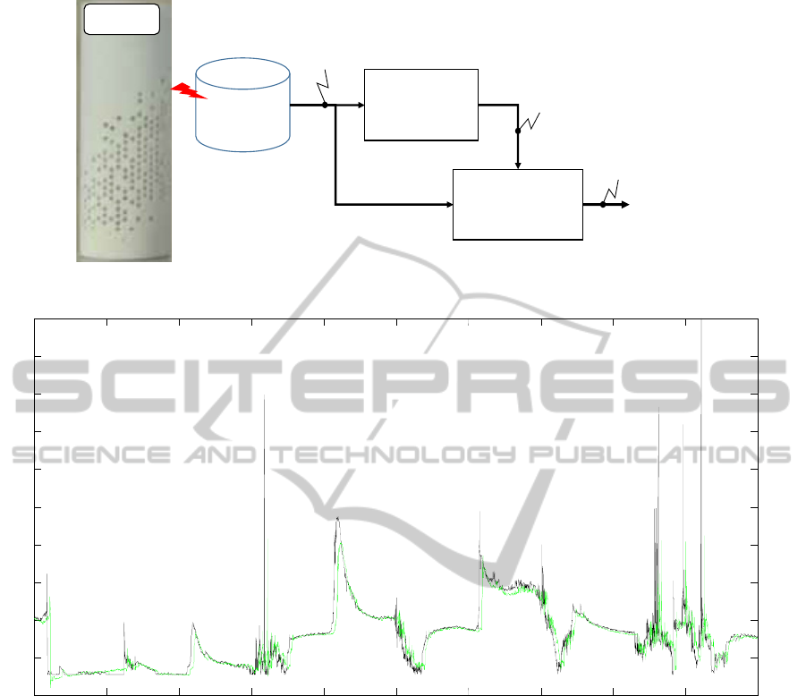
The figure 3 presents the principle of the prediction
of pollutants. The database collects data from the
Alima. These data are use in a first step in order to
detect the current situation (cooking, sleeping…)
which may have an impact on the pollutant
evolution. The design of the classification model has
already been submitted to the MOSIM2014
conference. This article is thus entirely focused on
the prediction model. This model takes as inputs the
8 actual outputs of the classification model and the 5
NCTA2014-InternationalConferenceonNeuralComputationTheoryandApplications
176

past values (
t, t-1, t-2, t-3, t-4) of the parameters
collected by Alima. Three different models are built
for each pollutant (CO
2
, COV, pm). The output of
the considered model is the value of the considered
pollutant 30 minutes later (
t+30). In order to avoid
the local minimum trapping, the learning is
performed on 20 different initial parameters sets.
The data set is divided in two subsets (learning and
validation data set) each corresponding to 15 days of
collected data. Only data collected by Alima1 are
used for the learning and validation. A pruning
algorithm is used in order to avoid the overfitting
problem. At last, the best resulting model is selected.
5 RESULTS
5.1 Results Obtained on the Validation
Data Set
In a first step, the results obtained on the validation
data set are presented. Figure 4 presents the
prediction of CO
2
(in green) to compare to the real
values collected (in black). This figure shows that
the evolution of CO2 level may be predicted with a
good accuracy even if the amplitude of the larger
variation can’t be predicted.
The figure 5 presents the prediction error for the
CO
2
pollutant (for the first 5 days of the validation
data set). This figure shows that the model is able to
predict the smooth evolution but it is not able to find
the total amplitude of greatest variations. For these
two figures, the data are normalized due to
confidential needing. However, the model works
with the true range of variation.
0 1 2 3 4 Day
-0.4
-0.2
0
0.2
0.4
0.6
0.8
Prediction
Error on CO
2
Figure 5: prediction error of C0
2
.
The results obtained for the COV pollutant is
quite similar and are not presented here.
Figure 6 and 7 present the same results obtained
for pm pollutants.
These two figures show that pm is corrupted with
an important noise. The events to detect have an
amplitude of the same order to the noise variance.
0 1 2 3 4 Day
0.65
0.7
0.75
0.8
0.85
0.9
0.95
pm
Figure 6: prediction of pm.
However, the model is able to predict the evolution
of the pm pollutant with a good accuracy.
5.2 Adaptation of the Models
The main goal of this model is to be suitable even if
the conditions change (move in the house, or change
of house …) and the model must to be portable from
one Alima to another. In order to do that, the model
must be adaptable on-line. To do that, we propose to
detect if the model varies from the reality, and to
perform a relearning only if needed.
0 1 2 3 4 Day
-0.15
-0.1
-0.05
0
0.05
0.1
0.15
0.2
0.25
0.3
Prediction
Error on pm
Figure 7: prediction error of pm.
In order to illustrate this, the preceding models
constructed with the data collected by airbox1 are
used with the data collected on airbox2.
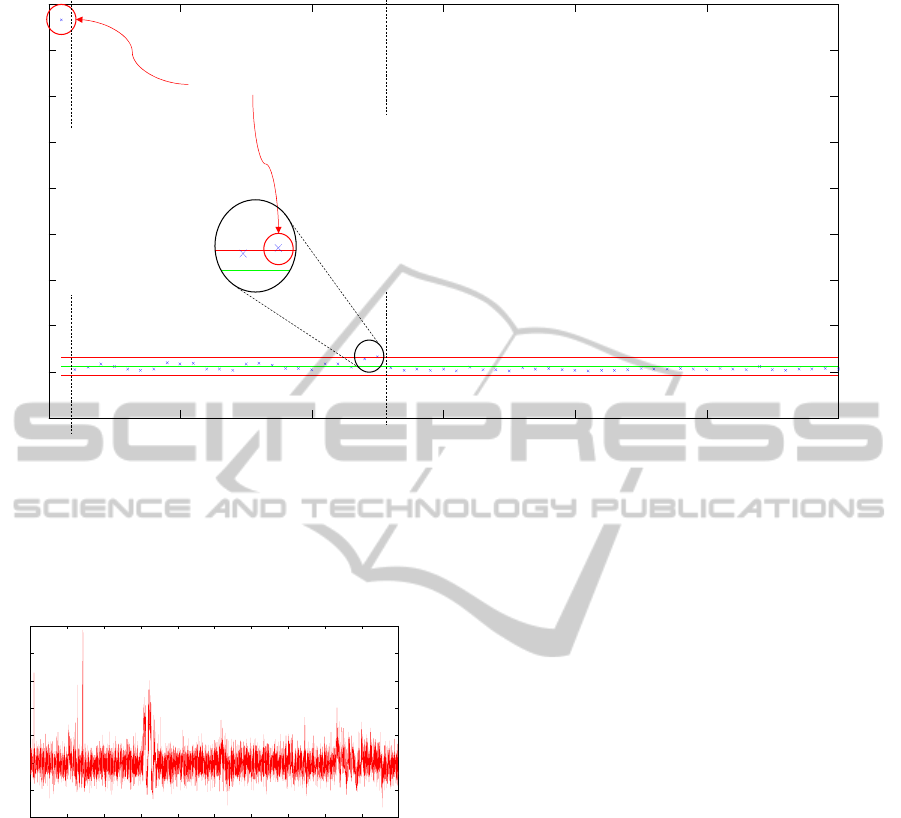
The s-chart described part 3 is used in order to
determine if a relearning is needed. The size of the
samples is fixed to 240 minutes and so each sample
contains 240 patterns. Figure 8 presents the s-chart
obtained for the pm model used with data collected
by airbox2.
This figure shows that, as awaited, the model is
not accurate for the first sample of 240 data. So a
relearning occurs on these 240 first data. This
relearning allows to fit the model to these new
condition and the model accuracy is satisfactory
until the sample 25. For this sample, the value of the
standard deviation is slightly outside the bounds and
a second relearning is needed. So, for the 15 days of
the experiments, only 2 relearning are needed to
PredictionModelAdaptationThankstoControlChartMonitoring-ApplicationtoPollutantsPrediction
177
0 10 20 30 40 50 sam
p
les
-200
0
200
400
600
800
1000
1200
1400
S-chart
UCL
LCL
Relearning needed
1
st
Relearning executed
2
nd
Relearning executed
Figure 8: S-chart: monitoring of model accuracy.
maintain a good accuracy of the model.
Figure 9 presents the prediction error for the pm
pollutant. This figure shows that this strategy allows
maintaining an accurate model even when the
conditions change.
0 1 2 3 4 Day
-0.2
-0.1
0
0.1
0.2
0.3
0.4
Prediction
Error on pm
Figure 9: prediction error of pm for airbox2.
6 CONCLUSIONS
This paper presents a new on-line monitoring
strategy conserving the prediction model accuracy.
This strategy is based on the use of a control chart to
determine if a relearning is needed or not to adapt
the model to an evolution of the reality. This
approach is tested on a prediction model related to
pollutants levels. The results show that neural
networks are able to predict the evolution of
pollutants. Moreover, the proposed monitoring
strategy allows adapting quickly the considered
model to new conditions and, in the same time, to
limit the number of relearning needed. In future
works, this approach will be compared with on-line
learning on both accuracy and computational time.
ACKNOWLEDGEMENTS
The authors thanks the society Anaximen for their
active financial and scientific support for this work.
REFERENCES
Alima, http://getalima.com, 2013.
Cybenko, G., 1989. Approximation by superposition of a
sigmoidal function. Math. Control Systems Signals, 2,
4, 303-314.
Du, L., Ke, Y., Su, S., 2012. The Embedded Quality
Control System of Product Manufacturing, Advanced
Materials Research, 459, 510-513.
Engelbrecht, A.P., 2001. A new pruning heuristic based on
variance analysis of sensitivity information. IEEE
transactions on Neural Networks, 1386-1399
Funahashi, K., 1989. On the approximate realization of
continuous mapping by neural networks. Neural
Networks, 2, 183-192.
Han, H.G., Qiao, J.F., 2013. A structure optimisation
algorithm for feedforward neural network
construction. Neurocomputing, 99, 347-357.
Heskes, T., Wiegerinck, W., 1996. A theoretical
comparison of batch-mode, online, cyclic, and almost-
cyclic learning. IEEE Transactions on Neural
Networks, 7, 919-925.
Jones, A.P, 1999. Indoor air quality and health.
Atmospheric Environment, 33, 28, 4535-4564.
NCTA2014-InternationalConferenceonNeuralComputationTheoryandApplications
178

Liang, N.Y., Huang, G.B., Saratchandran, P., Sundarajan,
N., 2006. A fast and accurate online sequential
learning algorithm for feedforward networks. IEEE
Transactions on Neural Networks, 17, 1411-1423.
Ma, L., Khorasani, K., 2004. New training strategies for
constructive neural networks with application to
regression problems. Neural Network, 589-609.
Maroni, M., Seifert, B., Lindvall, T., 1995. Indoor Air
Quality – a Comprehensive Reference Book. Elsevier,
Amsterdam.
Nakama, T., 2009. Theoretical analysis of batch and on-
line training for gradient descent learning in neural
networks. Neurocomputing, 73, 151-159.
Nguyen, D., Widrow, B., 1990. Improving the learning
speed of 2-layer neural networks by choosing initial
values of the adaptative weights. Proc. of the Int. Joint
Conference on Neural Networks IJCNN'90, 3, 21-26.
NIST/SEMATECH, 2012. e-Handbook of Statistical
Methods, http://www.itl.nist.gov/div898/handbook/.
Setiono, R., Leow, W.K., 2000. Pruned neural networks
for regression. 6
th
Pacific RIM Int. Conf. on Artificial
Intelligence PRICAI’00, Melbourne, Australia, 500-
509
Shewhart, W.A., 1931. Economic Control of Quality of
Manufactured Product, Van Nostrand Reinhold
Company, Inc.: Princeton, NJ.
Spengler, J. D., Sexton, K., 1983. Indoor air pollution: a
public health perspective. Science, 221, 9-17.
Tague, N.R., 2004. The Quality Toolbox, 2nd Edition,
ASQ Quality Press, http://asq.org/learn-about-
quality/data-collection-analysis-
tools/overview/control-chart.html.
Thomas, P., Bloch, G., 1997. Initialization of one hidden
layer feedforward neural networks for non-linear
system identification. 15
th
IMACS World Congress on
Scientific Computation, Modelling and Applied
Mathematics WC'97, 4, 295-300.
Thomas, P., Bloch, G., Sirou, F., Eustache, V., 1999.
Neural modeling of an induction furnace using robust
learning criteria. Journal of Integrated Computer
Aided Engineering, 6, 1, 5-23.
Thomas, P., Suhner, M.C., Thomas, A., 2013. Variance
Sensitivity Analysis of Parameters for Pruning of a
Multilayer Perceptron: Application to a Sawmill
Supply Chain Simulation Model. Advances in
Artificial Neural Systems, Article ID 284570,
http://dx.doi.org/10.1155/2013/284570
Walsh, P.J., Dudney, C.S., Copenhaver, E.D., 1987.
Indoor air quality, ISBM 0-8493-5015-8.
PredictionModelAdaptationThankstoControlChartMonitoring-ApplicationtoPollutantsPrediction
179
