
Dynamic Analysis for Golf Swing using of Mode Synthetics Method
for Suggesting an Optimal Club
Kenta Matsumoto
1
, Nobutaka Tsujiuchi
1
, Takayuki Koizumi
1
, Akihito Ito
1
,
Masahiko Ueda
2
and Kosuke Okazaki
2
1
Department of Mechanical Engineering, Doshisha University, 1-3, Tataramiyakodani, Kyotanabe-city,
Kyoto, 610-0321, Japan
2
Research Dept.
Ⅱ
, Research & Development HQ. Sumitomo Rubber Industries,Ltd, 1-1,2-chome,
Tsutsui-cho, Chuo-ku, Kobe 651-0071, Japan
Keywords: Golf Club, Finite Element Method, Mode Synthetics Method, Inertia Force.
Abstract: Advance of measurement system permits the measurement of high accuracy data. This study proposes
analysis of shaft movement using this system. Firstly, we made a shaft model using finite element method
and a club head model as concentrated mass. Secondly, we reduced amount of calculation by applying
mode synthetics method. Input data for simulation is inertia force and torque calculated from swing data
that is measured by motion capturing system and is treated data manually. Finally, we simulated shaft
movement using these data, we cloud repeat shaft movement of face direction and toe direction.
1 INTRODUCTION
Golf is the sport that can enjoy valuable generation
of people. Victory or defeat of this sport is decided
by score that move a golf ball to fixed location.
Therefore players want to get a golf club that is able
to hit a golf ball more accuracy and more far for
improving their playing. This study focuses on
driver among some clubs because hitting with a
driver determines score. For this reason, club head
of driver was improved bigger and more reactive.
However, not only volume of head of the golf club
but also coefficient of the golf club was restricted
by the effect rule of the spring of the United States
golf society. Therefore, it is becoming hard to
differentiate golf clubs for clubs spec. Then, the
implementers of golf club increase the lineup of
shaft and it provides the club fits for an individual.
As one of techniques, “Database fitting” was
established by SRI. “Database fitting” is the method
that recommends adequate shaft to a player by
analyzing the swing using grip end sensor.
In the future, the implementers would like to
provide custom-made shaft for each golfer. In order
to make this idea possible, the implementers need to
repeat movement of shaft that don’t exist in the
lineup in swinging.
Some studies of prediction movement of shaft in
swinging have using multi body dynamics (Inoue,
2000,2004),using vibration feature (Iwatsubo,
1990).However, the study using multi body
dynamics needs huge amount of calculation because
that has iterative calculation on that simulation. The
study using vibration feature has smaller amount of
calculation then multi body dynamics, but its
simulation is calculated on 2-dimension and don’t
repeat realistic movement of shaft in swinging that
need for its prediction.
Wherein, we intend to simulate movement of
shaft by 3-dimension input data using motion
capture system and by small amount of calculation
applying mode synthetics method.
2 SIMULATION MODEL
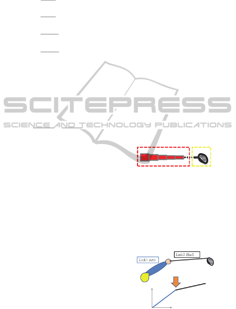
Simulation model of shaft is constructed with
multistage beam (Fig.1). Simulation model is
formulated by finite element method with beam type
element.
Figure 1: Simulation Model with Multistage Beam.
27
Matsumoto K., Tsujiuchi N., Koizumi T., Ito A., Ueda M. and Okazaki K..
Dynamic Analysis for Golf Swing using of Mode Synthetics Method for Suggesting an Optimal Club.
DOI: 10.5220/0005070700270033
In Proceedings of the 2nd International Congress on Sports Sciences Research and Technology Support (icSPORTS-2014), pages 27-33
ISBN: 978-989-758-057-4
Copyright
c
2014 SCITEPRESS (Science and Technology Publications, Lda.)
2.1 Beam Element
2.1.1 Displacement Function
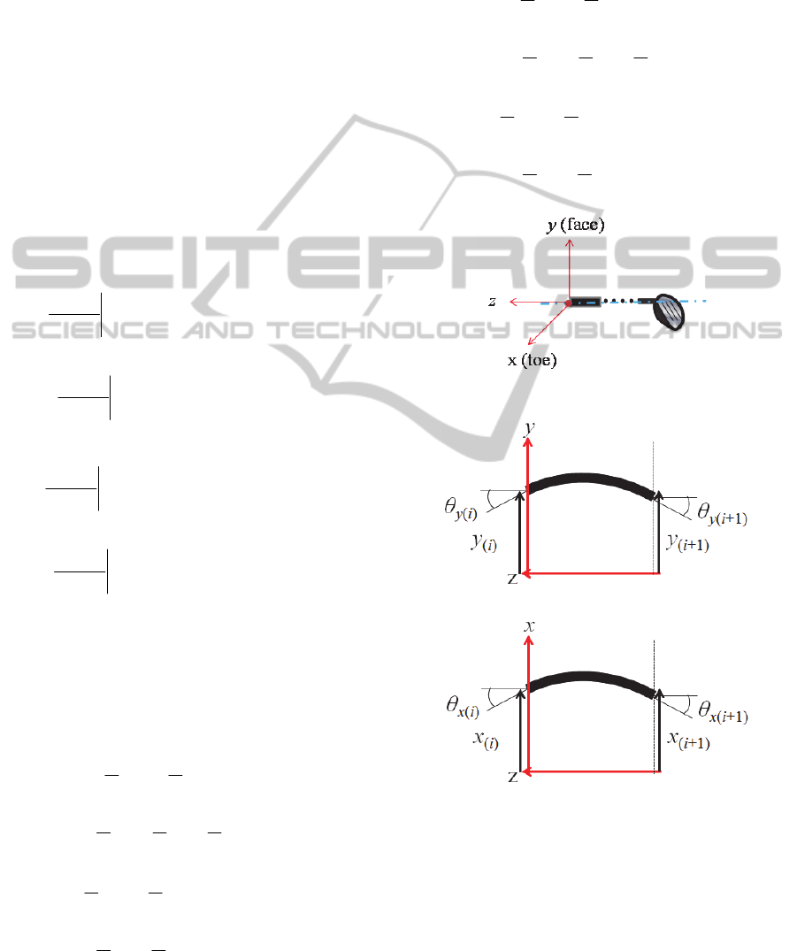
Coordinate system of shaft is defined as Fig.2. In
this study, x direction is defined as toe of club head
direction and y direction is defined as face of club
head direction. Displacement function of each
directions on this coordinate system is shown in
eq.(1), eq.(2).
3
3
2
210
, zazazaatzx
(1)
3
3
2
210
, zbzbzbbtzy
(2)
Deflection and deflection angle of each direction of
the i th element from grip end is defined as Fig.3,
deflection and deflection angle of each direction is
as follows.
2
3211
3
3
2
2101
1
0
0
32
,
,
LaLaa
dz
tzdx
LaLaLaax
a
dz
tzdx
ax
Lz
iy
i
z
iy
i
(3)
2
3211
3
3
2
2101
1
0
0
32
,
,
LbLbb
dz
tzdy
LbLbLbby
b
dz
tzdy
by
Lz
ix
i
z
ix
i
(4)
L is Element width. Each coefficients of eq.(1) and
eq.(2) are derived from eq.(3) and eq.(4).
)()]([),( tzNtzx
ixx
d
(5)
T
iyiiyiix
xxt ],,,[)(
11
d
(6)
32
4
32
3
32
2
32
1
4321
23
2
231
)]([
L
z
L
z
LN
L
z
L
z
N
L
z
L
z
L
z
LN
L
z
L
z
N
NNNNzN
x
x
x
x
xxxxx
(7)
)()]([),( tzNtzy
iyy
d
(8)
T
ixiixiiy
yyt ],,,[)(
11
d
(9)
32
4
32
3
32
2
32
1
4321
23
2
231
)]([
L
z
L
z
LN
L
z
L
z
N
L
z
L
z
L
z
LN
L
z
L
z
N
NNNNzN
y
y
y
y
yyyyy
(10)
Figure 2: Coordinate System of Shaft.
Figure 3: Each Deflection and Deflection angle.
2.1.2 Mass Matrix, Rigid Matrix
Motion energy of each directions T
x
, T
y
and potential
energy of each directions U
x
, U
y
are led as following
equations.
icSPORTS2014-InternationalCongressonSportSciencesResearchandTechnologySupport
28
dz
dt
tzdx
AT
L
x
0
2
,
(11)
dz
dt
tzdy
AT
L
y
0
2
,
(12)
0
2
2
2
,
L
xx
dz
dz
tzxd
EIU
(13)
0
2
2
2
,
L
yy
dz
dz
tzyd
EIU
(14)
A is cross-section area, ρ is density, E is Young’s
modulus, I
x
, I
y
are second moment of area. By
substituting eq.(5) and eq.(9) into eq.(11-14), we
obtain element mass matrix of each directions as
M
ele_x,y
and element rigid matrix of each directions as
K
ele_x,y
.
0
,,,_
][
L
yx
T
yxyxele
dzzNzNAM
(15)
d
z
dz
zNd
dz
zNd
EIK
L
yx
T
yx
yxyxele
0
2
,
2
2
,
2
,,_
)(
(16)
Index x,y of eq.(15) and eq.(16) show each direction.
By assembling these element matrixes, we compose
full mass matrix and full rigid matrix.
2.2 Equation of Motion
In this study, simulation model of shaft is divided
into 24 elements (Fig.1). By rearranging each
element matrixes, the i th element equation of
motion is composed as follows.
iiiiiii
tKtCtM fddd
(17)
11111
1
iyixiiie
iyixiiie
T
ieiei
yx
yx
t
d
d
ddd
(18)
Index (i) shows the i th
node
, f
(i)
is nodal force
acting of the i th
node,
d
(i)
(t) is nodal point
displacement, C
(i)
is damping matrix. Mass of club
head is added to final node as concentrated mass
.
Then, substituting element mass matrix on final
element as M
(n)
, the element of M
(n)
in the 1 row and
1 column and in the 2 th row and 2 column is as
follow equations.
headnelen
headnelen
MMM
MMM
2,22,2
1,11,1
(19)
M
e(n)
is the element mass matrix led from eq.(5),
M
head
is mass of club head. By assembling each
elements, full motion of equation is follow equation.
fddd tKtCtM
(20)
2.3 Mode Synthetics Method
Simulation model of shaft is divided into two area
that are c area and e area (Fig.4). By dividing its
model area, nodal point displacement and mass
matrix, rigid matrix are divided into each area. Then,
reduction matrix
t
T
is calculated. By multiplying
t
T
from the front of eq.(20), eq.(20) is reduced to
c
d
that shows area c and
ξ
that shows mode area
(Nagamatsu, 1985).
fTf
TKTK
TCTC
TMTM
fKCM
T
t
t
T
t
t
T
t
t
T
t
cc
~
~
~
~
~
~
~
~
ξ
d
ξ
d
ξ
d
c
(21)
Figure 4: Dividing Simulation Model into Each Area.
2.4 Input Data
In this study, we model swing movement as 2-link
model that is composed of arm and club for
repeating shaft movement (Fig.5). Shaft is modelled
by finite element method. Inertia force made by arm
movement is added to shaft in swinging. Therefore,
we need to calculate input data of this inertia force
for repeating shaft movement. The method of
calculating this input data is as follows.
Figure 5: 2 Link Model of Swing.
Area
e
Area
c
DynamicAnalysisforGolfSwingusingofModeSyntheticsMethodforSuggestinganOptimalClub
29
2.4.1 Coordinate System
We define a shoulder shown on Fig.5 as origin point
of inertial coordinate system [a]. Then, we define the
vector that shows from shoulder to shaft’s point of
union as r
0
and fixed coordinate system that origin
point is its point of union as [b].We also define the
vector that shows from this fixed coordinate
system’s origin point to the i th node as ρ
(i)
. And
then, by defining movement by elastic deformation
of the i th node as n
(i)
, the vector u
(i)
that shows from
inertial coordinate system to the i th node obtains as
follow.
iii
nρru
)(0
(22)
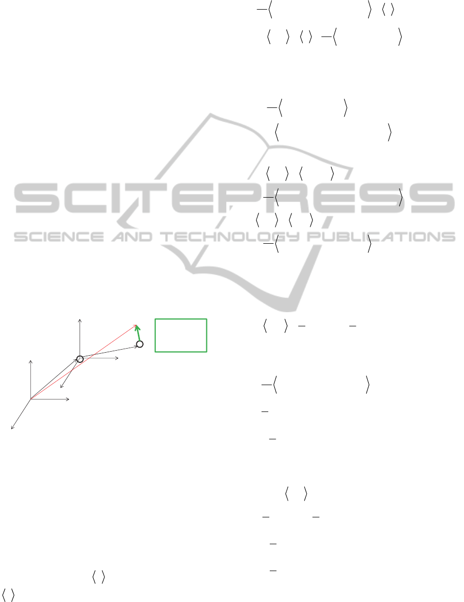
Each coordinate system and relationship of each
vector is shown on Fig.6. The relationship of each
coordinated system is obtained as follow.
Sab
(23)
S is coordinate transform matrix. Then, rate vector is
obtained as follow by eq.(22).
ini
iiii
vωr bba
nρrvu
~
ˆ
0
)(0
(24)
v
n(i)
is component of rate vector of the i th node, ω
~
is
angle rate tensor.
Figure 6: Each Coordinate System and Relationship of
Each Vector.
2.4.2 Input Force
Gravity vector g is shown by its component
g
ˆ
.
g
ˆ
ag
(25)
Then, we define linear momentum of the i th node as
P
(i)
and obtain follow equation by low of
conservation of liner momentum.
gP
i
(26)
shows integral of mass.By substituting
eq.(24)
into eq.(26), we obtain follow equation.
iin
ini
ωr
dt
d
a
vr
dt
d
~
ˆ
~
ˆ
0
0
bagb
gbωba
(27)
a
n(i)
is the component of acceleration vector of the i
th node on fixed coordinate system. Second on the
right-hand side of eq.(27) is deformed as follow.
ii
i
ωωωr
ωr
dt
d
~~~
ˆ
][
~
ˆ
0
0
bba
ba
(28)
Then, we deform eq.(28) by substituting eq.(23).
ii
T
T
in
ii
T
T
in
ωωωrS
d
t
d
gSa
ωωωrS
dt
d
gSa
~~~
ˆ
ˆ
~~~
ˆ
ˆ
0
0
bbb
bb
(29)
And then, by assuming inertia force that act to the i
th node is composed by each next element, the first
on the right-hand side of eq.(29) is explicated as
follow equation.
gSMgSMgS
T
i
T
i
T
ˆ
2
1
ˆ
2
1
ˆ
1
(30)
In a similar way, the second on the right-hand side
of eq.(29) is explicated as follow equation.
1101
0
0
~~~
ˆ
2
1
~~~
ˆ
2
1
~~~
ˆ
ii
T
i
ii
T
i
ii
T
ωωωrSM
ωωωrSM
ωωωrS
dt
d
(31)
Input force F
(i)
of the i th node is led from eq.(29-31)
as follow equation.
1101
0
1
~~~
ˆ
2
1
~~~
ˆ
2
1
ˆ
2
1
ˆ
2
1
ii
T
i
ii
T
i
T
i
T
i
ini
ωωωrSM
ωωωrSM
gSMgSM
aF
(32)
Especially, by considering influence of club head,
input force of final node is led as follow equation.
0
r
i
u
)(i
ρ
i
n
Position
Vector from
Each Node
[b]:Fixed
Coordinate
System
[a]:Inertial
Coordinat
e System
icSPORTS2014-InternationalCongressonSportSciencesResearchandTechnologySupport
30

headhead
T
head
nn
T
n
T
head
T
n
in
ωωωrSM
ωωωrSM
gSMgSM
aF
~~~
ˆ
~~~
ˆ
2
1
ˆˆ
2
1
0
0
(33)
2.4.3 Input Torque
We define the i th node circular torque as
i
T
.
ii
T
ˆ
aT
(34)
i
T
ˆ
is component of the i th node circular torque on
inertial coordinate system. Follow equations is led
by low of conservation of angular momentum.
0
ˆ
ˆˆ
~
ˆ
iii
Tgv
(35)
ii
Srv
~
ˆˆ
0
(36)
T
ii
SS
~
~
ˆ
(37)
STT
ˆ
(38)
i
~
is antisymmetrization tensor of fixed coordinate
vector
i
.Follow equation is led by explicating
eq.(38).
gTv
iii
ˆ
~
ˆ
ˆ
ˆ
~
ˆ
(39)
And then, the left-hand side of eq.(39) is explicated
by eq.(36) and eq.(37) as follow equation.
iii
T
ii
T
iii
T
ii
T
iiiii
SJJSrS
SJ
SrS
S
SrSv
~~
~
~~~~~~~
~~
~~~~
ˆ
~
ˆ
0
2
3
2
2
2
1
0
0)()(
(40)
T
iii
J
~
~
(41)
00
ˆ
rSr
(42)
00
ˆ
rSr
(43)
T
i 321
(44)
Component of torque vector on fixed coordinate
system is led by eq.(38-44) as follow equation.
gSJJrT
T
iiii
ˆ
~
~
~
0
(45)
In a similar way of input force, by assuming input
torque is composed by each next element, each
member of eq.(45) are explicated as follow equation.
gSMgSM
JJJJ
rMrMT
T
ii
T
ii
iiii
iiiii
ˆ
~
2
1
ˆ
~
2
1
2
1
2
1
~
2
1
~
2
1
~
2
1
~
2
1
11
11
0110
(46)
Especially, by considering influence of club head,
final node circular input torque is led as follow
equation.
gSMgSM
JJJJ
rMrMT
T
headhead
T
headhead
headhead
ˆ
~
ˆ
~
2
1
2
1
~~
2
1
~~
2
1
0
n
n
nn
nnnn
(47)
head
~
is the antisymmetrization tensor of the vector
that shows from final node to center of mass of
head,
head
J is inertia moment of head.
3 ANALYSIS METHOD
3.1 Measurement
Shaft movement in swinging was measured by 3D
motion capture system. Sampling frequency is
500[Hz], marker is attached on shaft as Fig.7. While,
we define coordinate system for measurement on
Fig.8.
Figure 7: Marker Location.
DynamicAnalysisforGolfSwingusingofModeSyntheticsMethodforSuggestinganOptimalClub
31
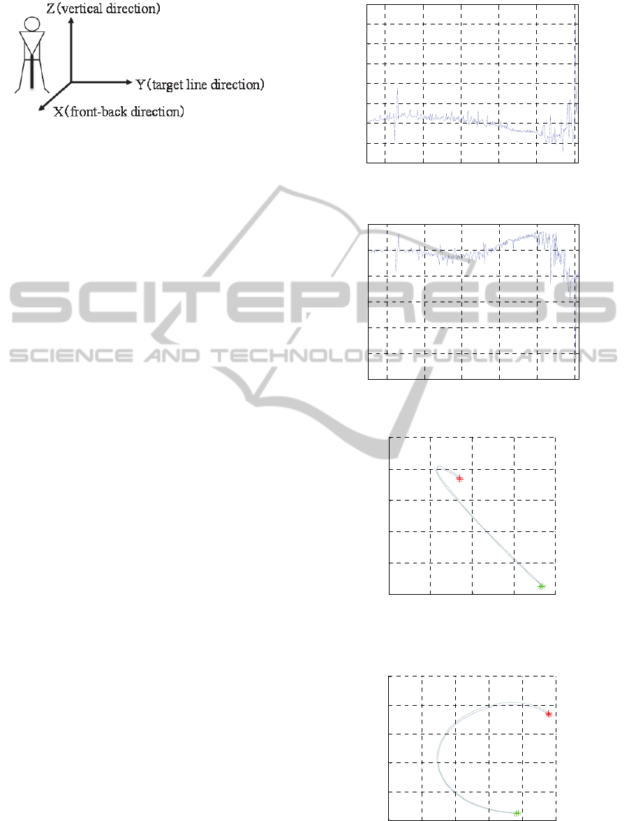
Figure 8: Coordinate System of Measurement.
3.2 Shaft Movement Prediction
Shaft movement was calculated by eq. (25) using
newmark β method. We added damping as adequate
numerical damping. Boundary condition was fixed
end, input data was calculated by eq. (32-33) and eq.
(46-47) using acceleration and angle rate, angle
acceleration data that have been obtained from
marker data of motion capture system. Acceleration
was led using by filtered motion data and Euler’s
approach. Angle rate and angle acceleration data is
led by quartanion. These programs were programed
by Matlab.
4 RESULTS AND DISCUSSION
We show each direction’s inertia force of shaft apex
calculated by motion data on Fig.9 with face
direction and Fig.10 with toe direction. And then, we
show movement of each direction of marker S5 in
close shaft apex on Fig.11 with vertical direction and
front-back direction, on Fig.12 with vertical
direction and target line direction. Blue line shows
motion and red line shows simulation data. Red
asterisk of Fig. (11-12) shows top of marker position
in swinging and lime green asterisk of Fig. (11-12)
shows the moment of impacting golf ball. By
showing Fig.11, there is the difference of about
0.035[m] motion line and simulation line near top.
However, by showing near impacting on Fig.11,
there is shorter difference of about 0.015[m] motion
line and simulation line near the moment of
impacting golf ball. Then, by showing Fig.12, there
is the difference of about 0.04 [m] motion line and
simulation line near top. However, by showing near
impacting on Fig.12, there is shorter difference of
about 0.015[m] motion line and simulation line near
the moment of impacting golf ball. For all of these
reasons, we concluded that we could repeat shaft
movement in swinging using by this simulation
model.
Figure 9: Inertia Force of Face Direction.
Figure 10: Inertia Force of Toe Direction.
Figure 11: Position Data as Viewing from behind target
line direction.
Figure 12: Position Data as Viewing from front - front-
back Direction.
-1 -0.8 -0.6 -0.4 -0.2 0
-40
-20
0
20
40
60
80
100
120
Time[s]
Force[N]
-1 -0.8 -0.6 -0.4 -0.2 0
-100
-80
-60
-40
-20
0
20
Time[s]
Force[N]
-2 -1.5 -1 -0.5 0
0
0.5
1
1.5
2
2
.
5
Vertical Direction[m]
Front-Back Direction[m]
-2 -1.5 -1 -0.5 0 0.5
0
0.5
1
1.5
2
2.5
Vertical Direction[m]
Target Line Direction[m]
Y-Z top-imp
icSPORTS2014-InternationalCongressonSportSciencesResearchandTechnologySupport
32

5 CONCLUSIONS
In this study we modelled shaft by finite element
method. And then, we reduced amount of calculation
by applying mode synthetics method and simulation
model calculated input data for this model from
motion data. By using this simulation model and
input data, we concluded that we could repeat shaft
movement in swinging using by this simulation
model.
REFERENCES
Yoshio Inoue, Yoshihiro Kai, Tetsuya Tanioka, 2000,
Study on Dynamics of Golf Swing (Boundary
Condition and Elasticity of Shaft), the Japan Society of
Mechanical Engineering
Yoshio Inoue, Kyoko Shibata, Koichi Okayama, Kyoji
Totsugi, 2004, Effect of the shaft elasticity in golf
swing, the Japan Society of Mechanical Engineering
Takuzo Iwatsubo, Nobuki Konishi, Tetsuo Yamaguchi,
1990, Research on Optimum Design of a Golf Club,
the Japan Society of Mechanical Engineering
Akio Nagamatsu, 1985, Mode Analysis, baihukan, 4
th
edition, pp.215-216
DynamicAnalysisforGolfSwingusingofModeSyntheticsMethodforSuggestinganOptimalClub
33
