Auditory Features Analysis for BIC-based Audio Segmentation

Tomasz Maka

Faculty of Computer Science and Information Technology,

West Pomeranian University of Technology, Szczecin, Zolnierska 49, 71-210 Szczecin, Poland

Keywords:

Auditory Features, Audio Segmentation, Delta-BIC Segmentation.

Abstract:

Audio segmentation is one of the stages in audio processing chain whose accuracy plays a primary role in the

ﬁnal performance of the audio recognition and processing tasks. This paper presents an analysis of auditory

features for audio segmentation. A set of features is derived from a time-frequency representation of an input

signal and has been calculated based on properties of human auditory system. An analysis of several sets of

audio features efﬁciency for BIC-based audio segmentation has been performed. The obtained results show

that auditory features derived from different frequency scales are competitive to the widely used MFCC feature

in terms of accuracy and the number of detected points.

1 INTRODUCTION

An accurate determination of audio segment bound-

aries has important inﬂuence on the efﬁcacy of nu-

merous audio and speech processing tasks. As a result

of the segmentation stage, an input audio stream is de-

composed into slices with determined positions where

audio content has a different acoustical structure. The

process of audio segmentation employs the properties

of feature space obtained in the audio parametrization

stage.

The typical approaches for segmentation of acous-

tical data can be categorized into two main groups:

metric-based and model-based. The ﬁrst group in-

cludes techniques based on the distance measures be-

tween adjacent audio frames to evaluate acoustic sim-

ilarity and to determine boundaries of the segments.

Another group contains methods for data models

comparison. The most popular technique is based

on the model analysis approach where the maximum

likelihood is estimated and the decision of a change

is made using the Bayesian information criterion

(BIC) (Chen and Gopalakrishnan, 1998). Although

this method gives good performance in many seg-

mentation systems, model-selection algorithms have

rather high computational cost (Cheng and Wang,

2003). Additionally, the effectiveness of this segmen-

tation approach is dependent on the analysis window

selection and computational decomposition. Several

techniques to deal with these issues are presented in

(Cettolo and Vescovi, 2003) and (Cheng et al., 2008).

Other approach to audio stream segmentation is

a technique which exploits self-similarity decompo-

sition (Foote and Cooper, 2003). Such decomposi-

tion is performed by calculating an audio inter-frame

spectral similarity in order to create a similarity ma-

trix. The audio segment boundaries are calculated by

correlating the diagonal of the similarity matrix with a

dedicated kernel. The obtained correlation result rep-

resents the possible boundaries of the audio regions.

An accuracy of audio segmentation algorithms de-

pends on the properties of feature space: its dimen-

sionality and the type of acoustical features. More-

over, the accuracy may be improved by limiting the

number of possible acoustical groups and perform-

ing the segmentation process for specialized tasks

like speaker diarization, broadcast news segmenta-

tion, speech/music regions determination, etc.

Also, the important factors diminishing the seg-

mentation effectiveness for speech signals are the

acquisition conditions. In order to reduce the in-

ﬂuence of adverse conditions on a particular seg-

mentation task, the robustness of features to noise

should be guaranteed. The compensation of the

background noise inﬂuence on the segmentation pro-

cess may be performed by using background mod-

els in the channel variability reduction process. For

example, in (Castan et al., 2013) a system based

on segmentation-by-classiﬁcation approach using the

compensation channel variability between the input

signal and acoustical background has been presented.

The main goal of this paper is the analysis and se-

Maka T..

Auditory Features Analysis for BIC-based Audio Segmentation.

DOI: 10.5220/0005063800480053

In Proceedings of the 11th International Conference on Signal Processing and Multimedia Applications (SIGMAP-2014), pages 48-53

ISBN: 978-989-758-046-8

 2014 SCITEPRESS (Science and Technology Publications, Lda.)

lection of the most discriminative audio features for

model-based audio segmentation. The paper is orga-

nized as follows. Section 2 describes auditory fea-

tures exploited in analysis. In Section 3 the well-

known technique called ∆BIC based on model anal-

ysis for audio segmentation is presented. Section 3

contains experimental results and discussion. The last

section concludes with the summary.

2 AUDIO FEATURES

In order to perform the audio segmentation phase,

a set of features describing the properties of sig-

nal changing signiﬁcantly between two different seg-

ments is required. Typically, in the majority of au-

dio segmentation systems the mel-frequency cepstral

coefﬁcients (MFCC) are used (Wu and Hsieh, 2006;

Xue et al., 2010; Chen and Gopalakrishnan, 1998).

Because the feature space type determines the seg-

mentation performance, we have decided to perform

the feature space analysis for different popular and

new feature sets.

In our study, the set of features includes typical

descriptors like LFCC and LPC which are exploited

in speech analysis and recognition tasks (Rabiner and

Schafer, 2010). Furthermore, we have introduced the

BFB feature set, where we used the set of 24 band-

pass ﬁlters mapped onto the Bark scale (Smith, 2011).

Then for each ﬁlter output, an energy was computed

and used as a descriptor. As it was reported in (Shao

and Wang, 2009), the GFCC features outperforms the

MFCC features for speech recorded in adverse con-

ditions. Therefore, we have decided to include it in

our study. For the ﬁnal feature set we have proposed

several simple descriptors using auditory ﬁlter bank.

These features are based on signals obtained from the

ﬁlter output such as Hilbert envelope, instantaneous

phase and frequency. For these signals we have mea-

sured period, mean, standard deviation and maximum

values.

The process of auditory features extraction uses

the approach presented in (Wang and Brown, 2006),

where an input signal is decomposed into a set of au-

ditory channels using the bank of ﬁlters derived from

observation of an auditory periphery. The usage of

auditory ﬁlter bank is motivated by its robustness in

comparison to Fourier-based analysis for signals with

mixtures of different sound sources (Ghitza, 1994).

The auditory ﬁlter called gammatone has been de-

signed based on functional approach of basilar mem-

brane mechanics.

The gammatone ﬁlter is a bandpass ﬁlter with the

following impulse response (Cooke, 2005):

g(t) = t

n−1

· e

−b·t

· e

i·2·π· f

·t

, (1)

where: n is the ﬁlter order, b denotes bandwidth for

a given frequency using equivalent rectangular band-

width (ERB) and f

is the ﬁlter center frequency.

Assuming that m(t) represents the complex output

of an auditory ﬁlter at frequency f

, we have com-

puted the instantaneous phase ϕ(t), instantaneous fre-

quency f(t) and Hilbert envelope H(t) as follows:

ϕ(t) = arg[m(t)], (2)

f(t) =

2π

ϕ(t), (3)

H(t) = |m(t)|. (4)

Having obtained signals ϕ(t), f(t) and H(t) we

have calculated features 7–12 presented in Tab. 1. In

case of the GTACI feature, we have estimated the pe-

riod of the ﬁltered signal using a common approach

exploiting autocorrelation function and peak detec-

tor (Rabiner and Schafer, 2010).

Table 1: Feature sets used in the experiments.

# Feature Description

1 MFCC Mel frequency cepstral coef-

ﬁcients (Rabiner and Schafer,

2010)

2 BFB Bark frequency ﬁlter bank

(Smith, 2011)

3 LFCC Linear frequency cepstral coef-

ﬁcients (Rabiner and Schafer,

2010)

4 LPC Linear prediction coefﬁcients

(Rabiner and Schafer, 2010)

5 GFCC Gammatone frequency cepstral

coefﬁcients (Shao and Wang,

2009)

6 GTACI Autocorrelation-based period

estimator of ﬁlter output

7 GTFMN Mean of f(t)

8 GTFSD Standard deviation of f(t)

9 GTPMN Mean of ϕ(t)

10 GTPSD Standard deviation of ϕ(t)

11 GTPMX max[ϕ(t)]

12 GTEMX max[H(t)]

3 CHANGE POINT DETECTION

One of the most popular techniques for audio seg-

mentation called Delta-BIC is based on the approach

AuditoryFeaturesAnalysisforBIC-basedAudioSegmentation

presented in (Chen and Gopalakrishnan, 1998), where

the acoustic change detection uses the Bayesian infor-

mation criterion (BIC) model selection penalized by

the model complexity. The delta-BIC method com-

pares two models: a model with data coming from

a single Gaussian distribution N(µ, Σ) and with data

modeled by two Gaussians – N(µ

, Σ

) and N(µ

, Σ

The data for the second model is extracted by split-

ting the input data at speciﬁed position i to the left

and right-side windows as depicted in Fig. 1.

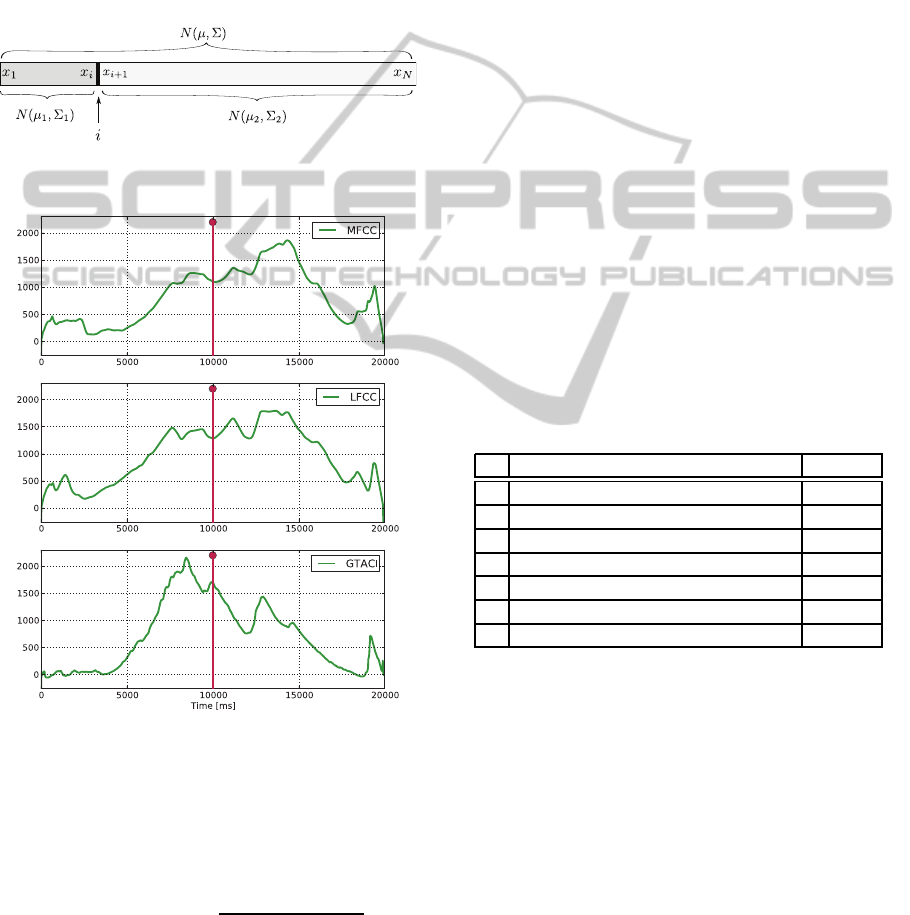
Figure 1: Data split in Delta-BIC segmentation scheme.

Figure 2: Delta-BIC trajectories calculated for the 6th di-

mensional feature space (d = 6) of the following features

(from top to bottom): MFCC, LFCC and GTACI.

The ∆BIC trajectory is computed as:

∆BIC(i) =N

(i)

log



(i)



− N

(i)

log



(i)



− Nlog|Σ| −

λ· logN · d(d + 3)

, (5)

where: N is the total length of analysed data window

, . . . , x

}, N

(i)

- the size of the left-side window

, . . . , x

}; N

(i)

- the size of the right-side window

i+1

, . . . , x

};



(i)



(i)



and



(i)



are determi-

nants of covariance matrices for the left-side, right-

side and the whole window; λ is a penalty weight

and d is a dimension of the feature space. Example

Delta-BIC trajectories for three different features are

depicted in Fig. 2. As it can be noticed, the type of

feature space is directly connected with the position

of the maximum value and thus it describes the oc-

currence of the change point. The maximum value of

∆BIC(i) determines a possible change point at posi-

tion argmax

∆BIC(i) when inequality max

∆BIC(i) >

0 is satisﬁed.

4 EXPERIMENTAL EVALUATION

The main purpose of the experiments was to deter-

mine which feature set gives the best results in de-

tecting a single change point in one audio data win-

dow using an analysis of ∆BIC trajectory. Thus, we

have used manually marked boundaries in broadcast

news database (Garofolo et al., 2004) as reference

points for segmentation. The characteristics of ex-

isting change points in available recordings from the

database is provided in Tab. 2.

Table 2: Types of segment boundaries in database (M/F –

Male/Female speech).

# Boundary type Occur.

1 music ↔ (M, F) / clean 10.9 %

2 (M, F) / clean ↔ (M, F) / mixture 5.7 %

3 (M) / clean ↔ (M) / clean 17.1 %

4 (F) / clean ↔ (M) / clean 20.6 %

5 (M) / clean ↔ (M, F) / noise 25.7 %

6 (F) / clean ↔ (M) / noise 4 %

7 (M) / noise ↔ (M, F) / noise 16 %

The prepared recordings in data set have length

20s, with one deﬁned change point after 10 second

each. The selected audio data had the sampling rate

22.5kHz/mono and the feature extraction process has

been done using a frame length equal to 30ms with

50% overlapping. In our experiments we have used

n = 4 order of the gammatone ﬁlter (Eq. 1) for audi-

tory features calculation and the penalty weight λ = 1

(Eq. 5) in the segmentation stage. We have per-

formed the experiment where all feature sets (Tab. 1)

have been used to calculate ∆BIC and to detect the

segment boundary. We have changed the number

of features in a single set from 1 to 24 and de-

termined the position of the change point. Due to

the same length of each audio example, the change

SIGMAP2014-InternationalConferenceonSignalProcessingandMultimediaApplications

1 3 5 7 9 11 13 15 17 19 21 23

0 5 10 15 20

MFCC BFB LFCC LPC GFCC GTACI

Feature vector size (d)

Change point position [s]

1 3 5 7 9 11 13 15 17 19 21 23

0 5 10 15 20

GTFMN GTFSD GTPMN GTPSD GTPMX GTEMX

Feature vector size (d)

Change point position [s]

(a)

1 3 5 7 9 11 13 15 17 19 21 23

0 5 10 15 20

MFCC BFB LFCC LPC GFCC GTACI

Feature vector size (d)

Change point position [s]

1 3 5 7 9 11 13 15 17 19 21 23

0 5 10 15 20

GTFMN GTFSD GTPMN GTPSD GTPMX GTEMX

Feature vector size (d)

Change point position [s]

(b)

1 3 5 7 9 11 13 15 17 19 21 23

0 5 10 15 20

MFCC BFB LFCC LPC GFCC GTACI

Feature vector size (d)

Change point position [s]

1 3 5 7 9 11 13 15 17 19 21 23

0 5 10 15 20

GTFMN GTFSD GTPMN GTPSD GTPMX GTEMX

Feature vector size (d)

Change point position [s]

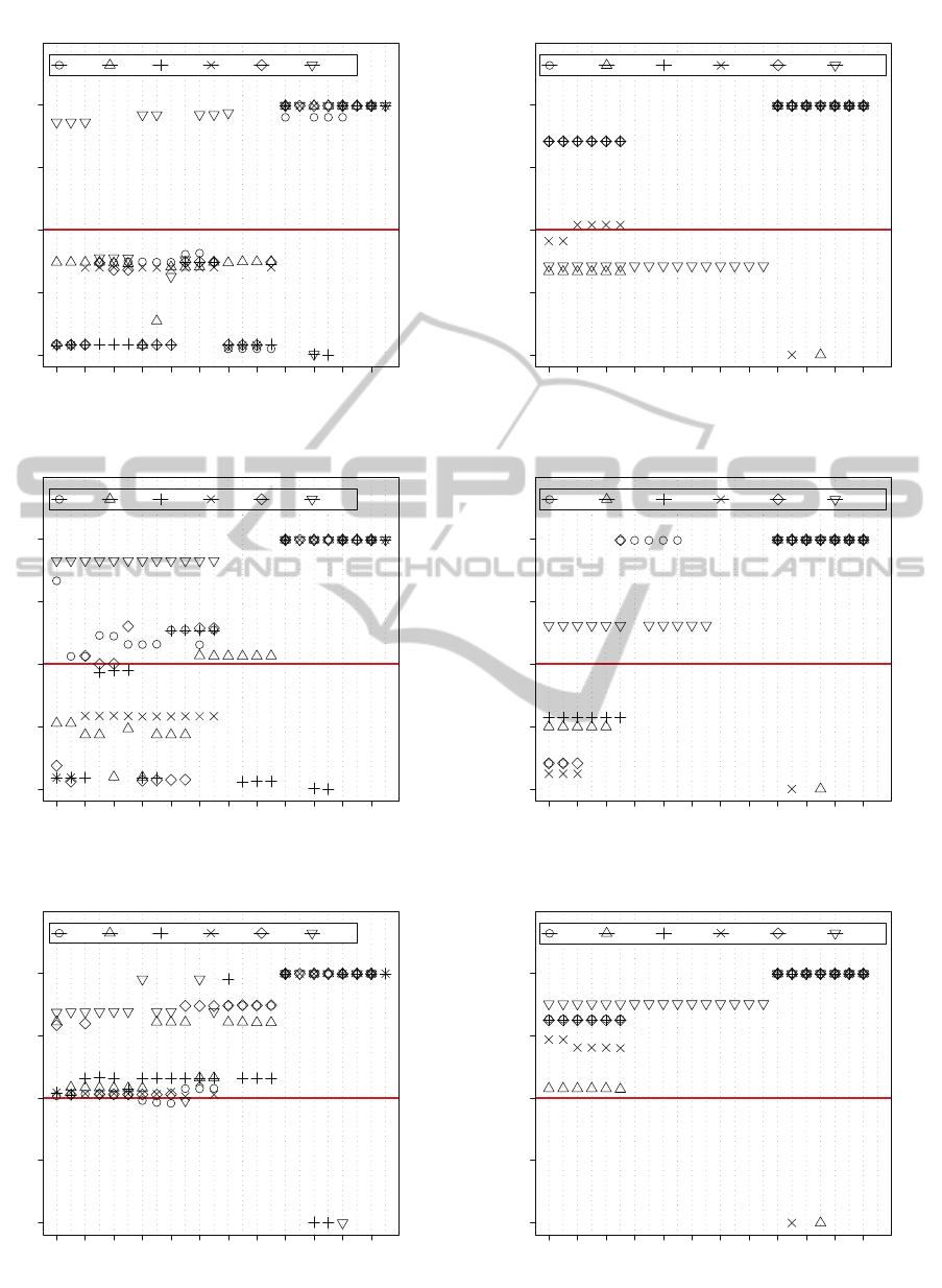
(c)

Figure 3: Positions of detected change points using all features for three example segments: speech (M) / clean → speech (M)

/ clean (a), speech (M) / clean → speech (F) / noise (b) and speech (F) / clean → speech (M) / clean (c).

AuditoryFeaturesAnalysisforBIC-basedAudioSegmentation

0 5 10 15 20

MFCC

BFB

LFCC

LPC

GFCC

GTACI

GTFMN

GTFSD

GTPMN

GTPSD

GTPMX

GTEMX

Change point [s]

Figure 4: Distribution of detected positions between two segments for the whole analysed data.

point should occur at the same position in each case.

The obtained results for three examples are shown

in Fig. 3, where the horizontal line denotes the de-

ﬁned change point. The best accuracy of the detected

points for the ﬁrst example (Fig. 3a) has been obtained

for GTPSD (d = 3, 4, 5, 6), second example (Fig. 3b)

has been observed for GFCC (d = 4, 5) and in the

last case (Fig 3c) for MFCC, LPC, LFCC and GFCC

(d = 1, . . . , 12). In case of all the examples, the statis-

tics of the detection accuracy are presented in Fig. 4

where the cross symbol denotes the arithmetic mean.

0 10 20 30 40 500 5 10 15 20 25 30 35 40 45 50

MFCC

BFB

LFCC

LPC

GFCC

GTACI

GTFMN

GTFSD

GTPMN

GTPSD

GTPMX

GTEMX

Missed change points [%]

Figure 5: The percentage of missed change points for each

set of features.

As a quality indicator of the differences between

positions of change points, the mean square error has

been used. In Fig. 6 the mean squared errors for

change point at position equal to 10 second are de-

picted. In this case, the best and the worst results have

been obtained for BFB and GTPSD features, respec-

tively.

20 25 30 35 40 45 50 5520 25 30 35 40 45 50 55

MFCC

BFB

LFCC

LPC

GFCC

GTACI

GTFMN

GTFSD

GTPMN

GTPSD

GTPMX

GTEMX

Mean Squared Error

Figure 6: Total mean square error of the positions of the

change points for each tested feature.

As it can be seen, for features BFB, LFCC, LPC,

GTFSD and GTEMX, the mean value is close (less

than 3 seconds) to the actual change point. For that

reason the feature space for ∆BIC trajectory calcula-

tion should include a combination of such features.

In many cases change points have not been detected.

SIGMAP2014-InternationalConferenceonSignalProcessingandMultimediaApplications

Therefore, we have counted such cases and the result

is depicted in Fig. 5. The worst efﬁciency in terms of

missed change points has been observed for features

7–11 (Tab. 1). The features exploited in our study

represents the properties of frequency distribution of

the input signals at different frequency scales. Con-

sequently, due to the fact that the input data in our

study contains mostly speech, the features which ex-

hibit the variability details of speech signal have led

to the most promising results.

In the most cases the fact of change point detection

is more important than the obtained accuracy. Thus,

the selection of feature vector size together with the

selection of the feature type is signiﬁcant for the ﬁ-

nal performance of the segmentation process. Also,

the parametrization stage should be carefully conﬁg-

ured for the expected types of audio segments and the

target application.

5 CONCLUSIONS

In this paper an analysis of auditory features efﬁ-

ciency for BIC-based audio segmentation has been

performed. For several examples 12 feature sets have

been examined. As the result, the features BFB,

LFCC, GFCC, GTACI and the GTEMX give promis-

ing results and they are competitive to the MFCC fea-

ture widely used in many audio segmentation sys-

tems. Due to the variability of the content in seg-

ment boundaries, better results seem to be achieved

in case of using joint different features. Also, in typ-

ical segmentation algorithm, an analysis window se-

lection and moving strategy have an important inﬂu-

ence on the segmentation results. Furthermore, the

fusion and clustering methods of the obtained change

points may improve signiﬁcantly the result for sig-

nals with several audio classes. Finally, an analysis of

features based on cochleagram and correlogram with

generalized likelihood ratio (GLR) and Hotteling’s T

trajectories is the future subject.

ACKNOWLEDGEMENTS

This work was sponsored by the Polish National

Science Center under a research project for years

2011-2014 (grant No. N N516 492240).

REFERENCES

Castan, D., Ortega, A., Villalba, J., Miguel, A., and

Lleida, E. (2013). Segmentation-by-classiﬁcation sys-

tem based on factor analysis. In IEEE International

Conference on Acoustics, Speech and Signal Process-

ing (ICASSP), pages 783–787.

Cettolo, M. and Vescovi, M. (2003). Efﬁcient audio seg-

mentation algorithms based on the bic. In IEEE Inter-

national Conference on Acoustics, Speech and Signal

Processing (ICASSP 2003).

Chen, S. and Gopalakrishnan, P. (1998). Speaker, envi-

ronment and channel change detection and clustering

via the bayesian information criterion,. In In Proc.

DARPA Broadcast News Transcription and Under-

standing Workshop.

Cheng, S. and Wang, H. (2003). A sequential metric-based

audio segmentation method via the bayesian informa-

tion criterion. In Proceedings EUROSPEECH 2003,

Geneva, Switzerland.

Cheng, S., Wang, H., and Fu, H. (2008). Bic-based audio

segmentation by divide-and-conquer. In IEEE Inter-

national Conference on Acoustics, Speech and Signal

Processing (ICASSP 2008).

Cooke, M. (2005). Modelling Auditory Processing and Or-

ganisation. Cambridge University Press.

Foote, J. and Cooper, M. (2003). Media segmentation using

self-similarity decomposition. In SPIE Storage and

Retrieval for Multimedia Databases, volume 5021,

pages 167–175.

Garofolo, J., Fiscus, J., and Le, A. (2004). 2002 Rich Tran-

scription Broadcast News and Conversational Tele-

phone Speech. Linguistic Data Consortium.

Ghitza, O. (1994). Auditory models and human perfor-

mance in tasks related to speech coding and speech

recognition. IEEE Transactions on Speech Audio Pro-

cessing, 2:115–132.

Rabiner, L. and Schafer, W. (2010). Theory and Applica-

tions of Digital Speech Processing. Prentice-Hall, 1st

edition.

Shao, Y. and Wang, D. (2009). Robust speaker identiﬁca-

tion using auditory features and computational audi-

tory scene analysis. In IEEE International Conference

on Acoustics, Speech and Signal Processing (ICASSP

2009).

Smith, J. (2011). Spectral Audio Signal Processing. W3K

Publishing, 1st edition.

Wang, D. and Brown, G. J. (2006). Computational Auditory

Scene Analysis. John Wiley & Sons, Inc., 1st edition.

Wu, C. and Hsieh, C. (2006). Multiple change-point audio

segmentation and classiﬁcation using an mdl-based

gaussian model. IEEE Transactions on Audio, Speech,

and Language Processing, 14(2).

Xue, H., Li, H., Gao, C., and Shi, Z. (2010). Computation-

ally efﬁcient audio segmentation through a multi-stage

bic approach. In 3rd International Congress on Image

and Signal Processing (CISP2010).

AuditoryFeaturesAnalysisforBIC-basedAudioSegmentation