
Modelling Exitement as a Reaction to a Virtual 3D Face
Egidijus Vaškevičius, Aušra Vidugirienė and Vytautas Kaminskas
Faculty of Informatics, Vytautas Magnus University, Vileikos g. 8, Kaunas, Lithuania
Keywords: 3D Face, Human Emotions, Input-Output Model, Parameter Estimation, Prediction, Model Validation.
Abstract: This paper introduces a comparison of a linear and nonlinear one step predictive models that were used to
describe the relationship between human emotional signal – excitement – as a reaction to a virtual 3D face
feature – distance between eyes. An input-output model building method is proposed that allows building a
stable model with the least output prediction error. Validation was performed using the recorded signals of
six volunteers and the following measures: prediction error standard deviation, relative prediction error
standard deviation, and average absolute relative prediction error. Validation results of the models showed
that both models predict excitement signal in relatively high prediction accuracy.
1 INTRODUCTION
Lots of systems and classification methods are used
for emotion recognition problem, but not so many
systems and methods are used for emotion control in
virtual environment. For this purpose plenty of bio-
signals are used for human state monitoring. We use
EEG-based signals because of their reliability and
quick response (Sourina and Liu, 2011; Hondrou
and Caridakis, 2012).
We have investigated linear input-output
structure models for exploring dependencies
between virtual 3D face features and human reaction
to them in Vidugirienė et al. (2013) and Vaškevičius
et al. (2014). Four reaction signals were used:
excitement, meditation, frustration, and engagement/
boredom. It was shown that features of a virtual face
have the largest influence to human excitement
signal from the previously mentioned four human
reaction signals (Vaškevičius et al., 2013).
In this investigation we compare a linear and one
type nonlinear input-output models to describe the
dependencies between human reaction – excitement
signal – to a virtual 3D face feature – distance-
between-eyes.
2 OBSERVATIONS AND DATA
A virtual 3D face with changing distance between
eyes was used for input as stimulus (shown in a
monitor) and EEG-based pre-processed excitement
signal of a volunteer was measured as output
(Figure 1). The output signals were recorded with
Emotiv Epoc device that records EEG inputs from
14 channels (according to international 10-20
locations): AF3, F7, F3, FC5, T7, P7, O1, O2, P8,
T8, FC6, F4, F8, AF4 (Emotiv Epoc specifications).
A dynamic stimulus was formed from a changing
woman face. One 3D face created with Autodesc
MAYA was used as a “neutral” one (Figure 1, left).
Other 3D faces were formed by changing distance-
between-eyes in an extreme manner (Figure 2).
Figure 1: Input-Output scheme for the experiments.
Figure 2: A 3D virtual face with the smallest (left), normal
(middle) and the largest (right) distance-between-eyes.
The transitions between normal and extreme
734
Vaškevi
ˇ
cius E., Vidugirien
˙
e A. and Kaminskas V..
Modelling Exitement as a Reaction to a Virtual 3D Face.
DOI: 10.5220/0005062907340740
In Proceedings of the 11th International Conference on Informatics in Control, Automation and Robotics (ICINCO-2014), pages 734-740
ISBN: 978-989-758-039-0
Copyright
c
2014 SCITEPRESS (Science and Technology Publications, Lda.)

stages were programmed.
Experiment plan for input is shown in Figure 3.
At first “neutral” face (Figure 2, middle) was shown
for 5 s, then the distance-between-eyes was
increased continuously and in 10 s the largest
distance between eyes (Figure 2, right) was reached,
then 5 s of steady face was shown and after that the
face came back to “normal” in 10 s. Then “normal”
face was shown for 5 s, followed by 10 s long
continuous change to the face with the smallest
distance between eyes (Figure 2, left), again 5 s of
steady face was shown and in the next 10 s the face
came back to “normal”. Then everything was
repeated from the beginning using 3 s time intervals
for steady face and 5 s for continuous change.
“Neutral” face has 0 value, largest distance-between-
eyes corresponds to value 3 and smallest distance-
between-eyes corresponds to value -3.
Values of the output signal – excitement – vary
from 0 to 1. If excitement is low, the value is close
to 0 and if it is high, the value is close to 1. The
signals were recorded with the sampling period of
T
0
=0.5 s.
Six volunteers (three females and three males)
were tested. Their excitement signals are shown in
Figures 4-5.
Figure 3: Input signal: experiment plan.
Figure 4: Excitement signal, volunteers no. 1-3 (females).
Figure 5: Excitement signal, volunteers no. 4-5 (males).
Each volunteer was watching one animated scene of
approximately 100 s, and EEG-based signals were
measured and recorded simultaneously.
3 BUILDING OF
MATHEMATICAL MODELS
Dependency between virtual 3D face feature
(distance-between-eyes) and human excitement is
described by input-output structure linear and
nonlinear models (Kaminskas, 1982) in (1) and (2)
correspondingly:
(1)
and
|
|
(2)
where
,
1
(3)
is an output (excitement),
is an input (distance-
between-eyes) signal respectively expressed as
,
(4)
with sampling period
,
is a constant value,
corresponds to noise signal, and z
-1
is the backward-
0 25 50 75 100
-2
0
2
Time, s
0 25 50 75 100
0
0.5
1
V
olunteer no.1
Time, s
0 25 50 75 100
0
0.5
1
Volunteer no.2
Time, s
0 25 50 75 100
0
0.5
1
Volunteer no.3
Time, s
0 25 50 75 100
0
0.5
1
Volunteer no.4
Time, s
0 25 50 75 100
0
0.5
1
Volunteer no.5
Time, s
0 25 50 75 100
0
0.5
1
Volunteer no.6
Time, s
ModellingExitementasaReactiontoaVirtual3DFace
735

shift operator (z
x
x
). A sign
||
denotes
absolute value.
These type of models were chosen to examine if
a volunteer reacts to the changes of a 3D face
(increase or decrease of distance-between-eyes)
directly (model 1) or he/she reacts to the absolute
values of the changes (model 2).
Parameters (coefficients of the polynomials (3)),
orders (degrees m and n of the polynomials (3)) and
constant
of the models (1) or (2) are unknown.
They have to be estimated according to the
observations obtained during the experiments with
the volunteers.
Eqs. (1) and (2) can be expressed in the
following forms:
,
(5)
,
(6)
It is not difficult to see that eqs. (5) and (6) can be
expressed as the linear regression equations:
+
(7)
where
1,
,
,…,
,
,…,
(8)
for model (1),
1,
|
|
,
|
|
,…,
|
|
,
,…,
(9)
for model (2), and
,
,
,…,
,
,
,…,
,
(10)
for both models, and T is a vector transpose sign.
For the estimation of unknown parameter vector
c we use a method of least squares (Kaminskas,
1982):
,
(11)
where and are expressed as follows
,
(12)
,
(13)
and M is a number of observation values that are
used to build a model.
After calculating the estimates of model
parameters, model’s stability condition is verified
(Kaminskas, 1982). It means that the roots
:
0,1,2,…,
(14)
of the following polynomial
(15)
have to be in the unit disk
1.
(16)
Estimates of the model orders – and – are
defined from the following conditions (Kaminskas,
1982):
:
,1
,
,
,
1,2,…
(17)
:
1,
,
,
,
0,1,…,
(18)
where
,
1
̂
,
(19)
is one step output prediction error standard
deviation,
̂
,
|
,
(20)
is one step output prediction error,
|
1
(21)
is one step forward output prediction in the case of
model (1) and
|
1
|
|
(22)
in the case of model (2) (Kaminskas, 2007), z is the
forward-shift operator (zy
y
), and 0 is a
chosen constant value. Usually in the practice of
identification ∈0,0010,01 what corresponds
to a relative variation of prediction error standard
deviation from 0,1% to 1%.
This way stable input-output models are built
that ensure the best one step output signal prediction.
ICINCO2014-11thInternationalConferenceonInformaticsinControl,AutomationandRobotics
736
4 VALIDATION OF PREDICTIVE
MODELS
Validation of the models (1) and (2) was performed
for each of six volunteers (three female and three
male).
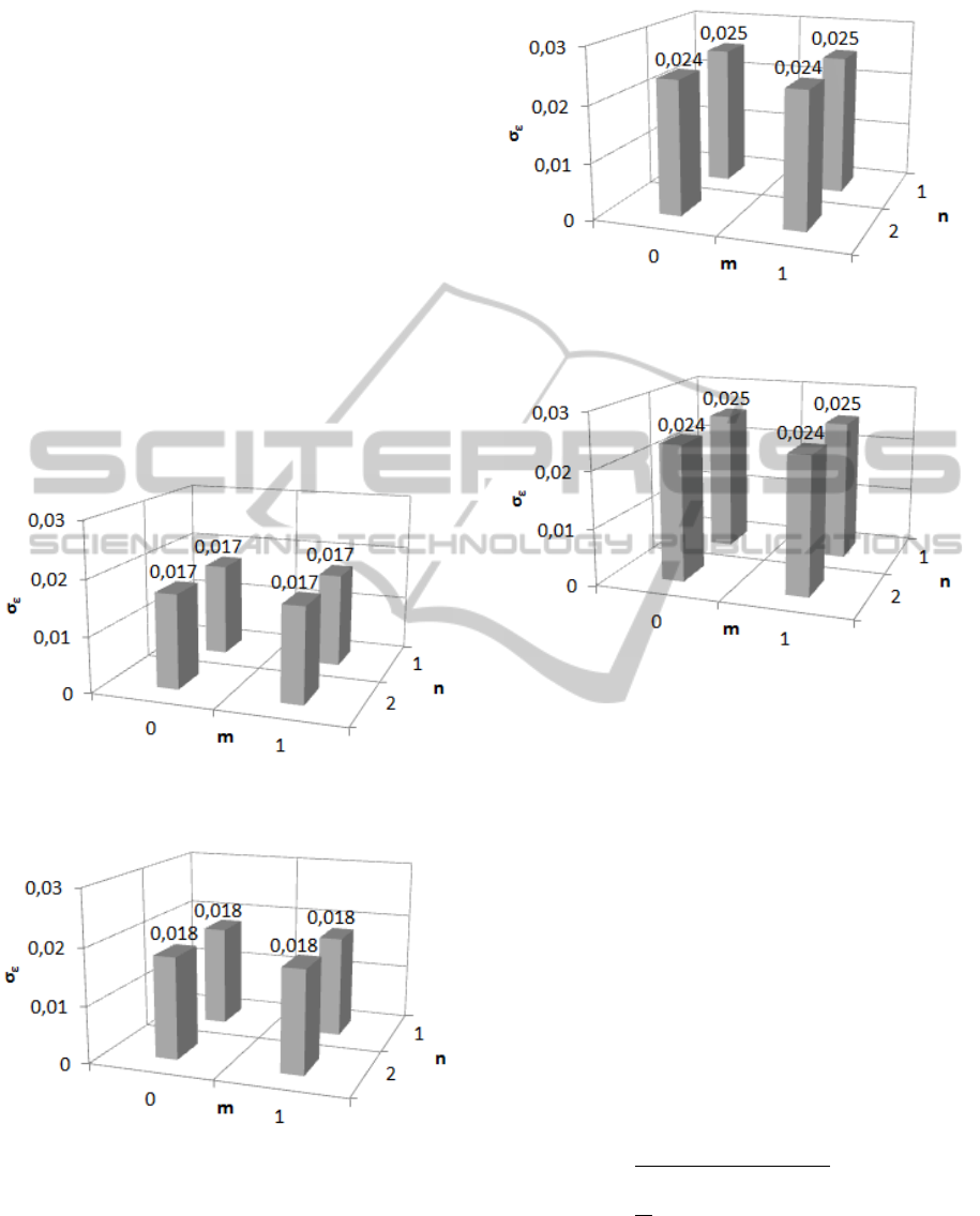
Figs. 6-9 demonstrate prediction error standard
deviations for an input-output pair when n=1, 2 and
m=0, 1, for one male (volunteer no.4) and one
female (volunteer no.2) using model (1) and
model (2).
Each model is selected from four possible
models (when n=1, 2; m=0, 1) using the rules (17)
and (18).
The analysis of two volunteers’ data showed that
relations between distance-between-eyes input and
excitement output signal can be modelled when
model order is 0, and 1.
Figure 6: Prediction error standard deviations with
different model (1) orders for a volunteer no. 2 (female).
Figure 7: Prediction error standard deviations with
different model (2) orders for a volunteer no. 2 (female).
Figure 8: Prediction error standard deviations with
different model (1) orders for a volunteer no. 4 (male).
Figure 9: Prediction error standard deviations with
different model (2) orders for a volunteer no. 4 (male).
The predicted output signals of every model have
the following expressions (Kaminskas, 1982)
|
1
(23)
in the case of model (1) and
|
1
|
|
|
|
(24)
in the case of model (2).
Prediction accuracies were evaluated using the
following measures:
prediction error standard deviation
1
|
,
(25)
relative prediction error standard deviation
ModellingExitementasaReactiontoaVirtual3DFace
737

1
|
∗100%,
(26)
and average absolute relative prediction
error
|
̅
|
1
|
∗100%.
(27)
Predictions were performed using the observation
data that were used to build a model (M=124, in (12)
and (13)) and the additional ones that were not used
to build a model (N=200, in (25)-(27)). Prediction
accuracies and parameters of the models are
provided in Table 1 and Table 2 for female and male
volunteers respectively.
Table 1: Prediction errors and model parameter estimates
for the volunteers no. 1-3 (females).
Volunteer
no.
Model
,
%
|
|
,
%
b
0
a
1
1 1 0.0246 4.46 6.59 -0.0014 -0.9856 0.0006
2 0.0246 4.47 6.57 -0.0018 -0.9822 0.0036
2 1 0.0174 3.51 5.63 0.0007 -0.9097 0.0085
2 0.0176 3.55 5.69 -0.0006 -0.9099 0.0093
3 1 0.0271 5.23 7.94 -0.0002 -0.8676 0.0399
2 0.0275 5.32 8.13 -0.0029 -0.8574 0.0469
Figures 10-15 show prediction results when using
linear model (1) for all six volunteers. Thin solid
line denotes an observed signal and thick dotted line
denotes predicted signal.
Table 2: Prediction errors and model parameter estimates
for the volunteers no. 4-6 (males).
Volunteer
no.
Model
,
%
|
|
,
%
b
0
a
1
4 1 0.0248 4.64 7.21 0.0012 -0.9139 0.0189
2 0.0253 4.75 7.43 -0.0042 -0.8898 0.0303
5 1 0.0258 5.12 8.26 0.0005 -0.9594 0.0066
2 0.0260 5.19 8.68 -0.0088 -0.9362 0.0251
6 1 0.0245 4.80 7.94 -0.0001 -0.9674 0.0079
2 0.0249 4.91 8.09 -0.0040 -0.9869 0.0079
Vertical thin dotted line denotes M position as
model parameters were estimated in the interval
from 0 to M (that is equal to 124). As the signal was
measured with the sampling period of T
0
=0.5 s, M
value corresponds to 62 s.
Figure 10: Prediction error standard deviations for
volunteer no. 1 (female). Thin solid line denotes a real
observed signal and thick dotted line denotes predicted
signal. Vertical thin dotted line denotes M position.
Figure 11: Prediction error standard deviations for
volunteer no. 2 (female). Thin solid line denotes a real
observed signal and thick dotted line denotes predicted
signal. Vertical thin dotted line denotes M position.
Figure 12: Prediction error standard deviations for
volunteer no. 3 (female). Thin solid line denotes a real
observed signal and thick dotted line denotes predicted
signal. Vertical thin dotted line denotes M position.
25 50 75 100
0
0.2
0.4
0.6
0.8
Time, s
Model building
25 50 75 100
0
0.2
0.4
0.6
0.8
Time, s
Model building
25 50 75 100
0
0.2
0.4
0.6
0.8
Time, s
Model building
ICINCO2014-11thInternationalConferenceonInformaticsinControl,AutomationandRobotics
738

Figure 13: Prediction error standard deviations for
volunteer no. 4 (male). Thin solid line denotes a real
observed signal and thick dotted line denotes predicted
signal. Vertical thin dotted line denotes M position.
Figure 14: Prediction error standard deviations for
volunteer no. 5 (male). Thin solid line denotes a real
observed signal and thick dotted line denotes predicted
signal. Vertical thin dotted line denotes M position.
Figure 15: Prediction error standard deviations for
volunteer no. 6 (male). Thin solid line denotes a real
observed signal and thick dotted line denotes predicted
signal. Vertical thin dotted line denotes M position.
5 CONCLUSIONS
Two alternative predictive models – linear and
nonlinear – were proposed to describe the
dependencies between 3D face feature (distance-
between-eyes) and excitement. The first model
describes the reaction of a volunteer to the direct
changes of a 3D face (increase or decrease of
distance-between-eyes). The second describes the
reaction of a volunteer to the absolute values of the
changes of a 3D face.
A method for building input-output models was
proposed that allows building stable models for the
predictions of excitement signals with the least
prediction error.
Validation of the models showed that each
volunteer has an individual reaction to the given
stimuli, and the reactions can be described using first
order (n=1, m=0) models. The absolute relative
predictions errors for the excitement signals are
between 5.5 % and 8.5 % in both model cases.
ACKNOWLEDGEMENTS
Postdoctoral fellowship of Ausra Vidugiriene is
funded by European Union Structural Funds project
”Postdoctoral Fellowship Implementation in
Lithuania” within the framework of the Measure for
Enhancing Mobility of Scholars and Other
Researchers and the Promotion of Student Research
(VP1-3.1-ŠMM-01) of the Program of Human
Resources Development Action Plan.
REFERENCES
Hondrou, C., Caridakis, G., 2012. Affective, Natural
Interaction Using EEG: Sensors, Application and
Future Directions. In Artificial Intelligence: Theories
and Applications, Vol. 7297, p. 331-338. Springer-
Verlag Berlin Heidelberg.
Emotiv Epoc specifications. Brain-computer interface
technology. Available at: http://www.emotiv.com/
upload/manual/sdk/EPOCSpecifications.pdf.
Kaminskas, V., 1982. Dynamic Systems Identification via
Discrete-Time Observations. Part1 – 1982, Part 2 –
1985. Vilnius: Mokslas. (in Russian).
Kaminskas, V., 2007. Predictor-based self tuning control
with constraints. In: Model and Algorithms for Global
Optimization, Optimization and Its Applications Vol.
4, p. 333-341. Springer.
Sourina, O., Liu, Y., 2011. A Fractal-based Algorithm of
Emotion Recognition from EEG using Arousal-
valence model. In Proc. Biosignals, p. 209-214.
25 50 75 100
0
0.2
0.4
0.6
0.8
Time, s
Model building
25 50 75 100
0
0.2
0.4
0.6
0.8
Time, s
Model building
25 50 75 100
0
0.2
0.4
0.6
0.8
Time, s
Model building
ModellingExitementasaReactiontoaVirtual3DFace
739

Vaškevičius, E., Vidugirienė, A., Kaminskas, V., 2013.
Investigation of dependencies between virtual 3D face
stimuli and emotion-based human responses. In: Proc.
of the 8th International Conference on Electrical and
Control Technologies, p. 64-69. Kaunas, Lithuania.
Vaškevičius, E., Vidugirienė, A., Kaminskas, V., 2014.
Identification of Human Response to Virtual 3D Face
Stimuli. Information Technologies and Control, Vol.
43, No. 1.
Vidugirienė, A., Vaškevičius, E., Kaminskas V., 2013.
Modeling of Affective State Response to a Virtual 3D
Face. In: UKSim-AMSS 7th European Modelling
Symposium on Mathematical Modelling and Computer
Simulation (EMS 2013), p. 167-172. Manchester, UK.
ICINCO2014-11thInternationalConferenceonInformaticsinControl,AutomationandRobotics
740
