Impedance Shaping Controller for Robotic Applications in Interaction
with Compliant Environments
Loris Roveda
1,2
, Federico Vicentini
1
, Nicola Pedrocchi
1
, Francesco Braghin
2
and Lorenzo Molinari Tosatti
1
1
Institute of Industrial Technologies and Automation (ITIA) of Italian National Research Council (CNR),
via Bassini, 15 - 20133 Milan, Italy
2
Politecnico di Milano, Department of Mechanical Engineering, via La Masa 1, 20156 Milan, Italy
Keywords:
Variable Impedance Control, Force-tracking Impedance Controls, Interacting Robotics Applications, Compli-
ant Environments.
Abstract:
The impedance shaping control is presented in this paper, providing an extension of standard impedance
controller. The method has been conceived to avoid force overshoots in applications where there is the need
to track a force reference. Force tracking performance are obtained tuning on-line both the position set-
point and the stiffness and damping parameters, based on the force error and on the estimated stiffness of
the interacting environment (an Extended Kalman Filter is used). The stability of the presented strategy
has been studied through Lyapunov. To validate the performance of the control an assembly task is taken
into account, considering the geometrical and mechanical properties of the environment (partially) unknown.
Results are compared with constant stiffness and damping impedance controllers, which show force overshoots
and instabilities.
1 INTRODUCTION
Robot machining and manipulation tasks require the
control of the interaction between the robot and the
surrounding environment, regardless the incomplete-
ness and/or inaccuracies in the knowledge of the stiff-
ness and location of the environment. In particular,
compliant environments, e.g. in surgical applications,
or high-added value materials could require a precise
control of critical interaction forces during a task ex-
ecution, e.g. avoiding force overshoots.
Principal methods for accomplishing robust and
safe interactions certainly involve compliance con-
trols. Since the milestones of sensor-based
force/dynamics control (Salisbury, 1980; Mason,
1981; Raibert and Craig, 1981; Yoshikawa, 1987;
Khatib, 1987; Yoshikawa and Sudou, 1990), dynamic
balance between controlled robots and environments
have primarily followed the approach of impedance
controls (Hogan, 1984), including also non-restrictive
assumptions (Colgate and Hogan, 1989) on the dy-
namical properties of the environment.
Impedance methods are proved to be dynami-
cally equivalent to explicit force controls (Volpe and
Khosla, 1995), but a direct tracking of explicit inter-
action forces or deformation is not straightforwardly
allowed. To overcome this limitation, preserving the
properties of impedance control, two different fami-
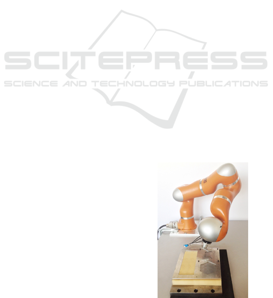
Figure 1: Experimental set-up for the assembly task execu-
tion.
444
Roveda L., Vicentini F., Pedrocchi N., Braghin F. and Molinari Tosatti L..
Impedance Shaping Controller for Robotic Applications in Interaction with Compliant Environments.
DOI: 10.5220/0005059504440450
In Proceedings of the 11th International Conference on Informatics in Control, Automation and Robotics (ICINCO-2014), pages 444-450
ISBN: 978-989-758-040-6
Copyright
c
2014 SCITEPRESS (Science and Technology Publications, Lda.)

lies of methods have been mainly introduced: (a) set-
point deformation and (b) variable impedance adapta-
tion.
For class (a), the most straightforward solution is
suggested in (Villani et al., 1999), where the time-
varying controlled force is derived from a position
control law, scaling the trajectory as a function of the
estimated environment stiffness. Another important
approach (Seraji and Colbaugh, 1997) involves the
generation of a reference motion as a function of the
force-tracking error, under the condition that the envi-
ronment stiffness is variously unknown, i.e. estimated
as a function of the measured force. Commonly in (a),
all approaches mantain a constant dynamic behaviour
of the controlled robot, so that when the environment
stiffness quickly and significantly changes, the bandi-
wth of the controllers has to be limited for avoiding
instability.
Class (b) methods introduce the modification of
the dynamic behaviour (i.e. online modification of
the impedance parameters) during the task execution.
Common solutions consist on gain
¯
/scheduling strate-
gies that select the stiffness and damping parame-
ters from a predefined set (off-line calculated) on the
basis of the current target state (Ikeura and Inooka,
1995; Ferraguti et al., 2013). Such approaches are
used in tasks characterized by a stationary, known and
structured environment. When the environment is un-
known or time-varying, the continuous adaptation of
the impedance parameters out of a tracking error en-
sures better perfomance (Dubey et al., 1997; Park and
Cho, 1998; Lee and Buss, 2000; Yang et al., 2011). To
the best of authors’ knowledge, no contributions are
given to the impedance adaptation taking into account
the runtime estimation of the environment stiffness.
Remarkably, the discussed classes of algorithms are
rarely applied in tasks where the environment proper-
ties change.
As a result, the main limitation in state-of-the-art
methods is in terms of reduced bandwidth (i.e. lim-
iting high perfomances) when the robot has to work
(e.g. to machine, assemble, etc) in contact to un-
structured and variable environments. Nevertheless,
there is a wide range of interacting robotic applica-
tions (Roveda et al., 2013) in which it is important to
estimate the environment dynamic parameters in or-
der to improve the controller performances.
The purpose of the presented work is to extend
the deformation/force-tracking impedance control to
a global impedance shaping. This class (b) strategy
introduces the ability to tune all impendance parame-
ters (velocity/position set-point, stiffness and damp-
ing) at runtime, using both the tracking error and
the estimate of the environment dynamic parameters.
Equivalently, the impedance of the global system con-
trolled robot-interacting environment is shaped to the
task (unforeseen) properties.
The goals of such defined control strategy are to
i) avoid force orvershoots that may damage the inter-
acting environment ii) in applications where there is
the need to track a force reference, iii) allowing max-
imum dynamic performance of the controlled robot.
In adapting the parameters, for instance, stiffness and
damping are defined as quadratic functions of the
force error. This choice allows the definition of both
high stiffness and low damping in the free space (in
order to have maximum performances of the con-
trolled robot to reach the target force reference) and
low stiffness and high damping during contacts (in or-
der to avoid force overshoots and to fit the dynamics
of the environment), satisfying Lyapunov stability re-
quirements.
The estimation of the environment stiffness is car-
ried out by implementing an Extended Kalman Fil-
ter (EKF) as in (Roveda et al., 2013). The dynamic
model of the interaction is based on a pure impedance
model for both the controlled robot and the interacting
compliant environment.
The effectiveness of the proposed control scheme
is tested using a KUKA LWR 4+ manipulator in an as-
sembly task (Figure 1). The task has been performed
without knowing the environment’s geometrical and
mechanical properties. An assembly task has been se-
lected due to its high relevance in industrial contexts.
2 PROBLEM FORMULATION
AND CONTROL MODEL
Based on the estimate of the environment dynamic
parameters and the force error e
f
= f
d
− f
r
, where
f
d
and f
r
are the desired and measured robot forces,
respectively, the impedance shaping control (Fig. 2)
defines the set-point ∆x
0
and the stiffness and damp-
ing matrices K,D of the robot impedance control in
order to shape the global impedance. A proportional
term is used in order to track the desired interacting
force. Stiffness and damping matrices are defined as
a quadratic function of the force error. Symbolically
K = K
0
+ m
K
e
2
f
(1)
D = D
0
+ m
D
e
2
f
(2)
∆x
0
= x + K
P
b
K
−1
e
e
f
(3)
b
K
e
= f (f
e
,x
eq
e
,x
e
) (4)
where K is the diagonal stiffness matrix of the con-
trolled robot, K
0
is the diagonal stiffness matrix of
ImpedanceShapingControllerforRoboticApplicationsinInteractionwithCompliantEnvironments
445
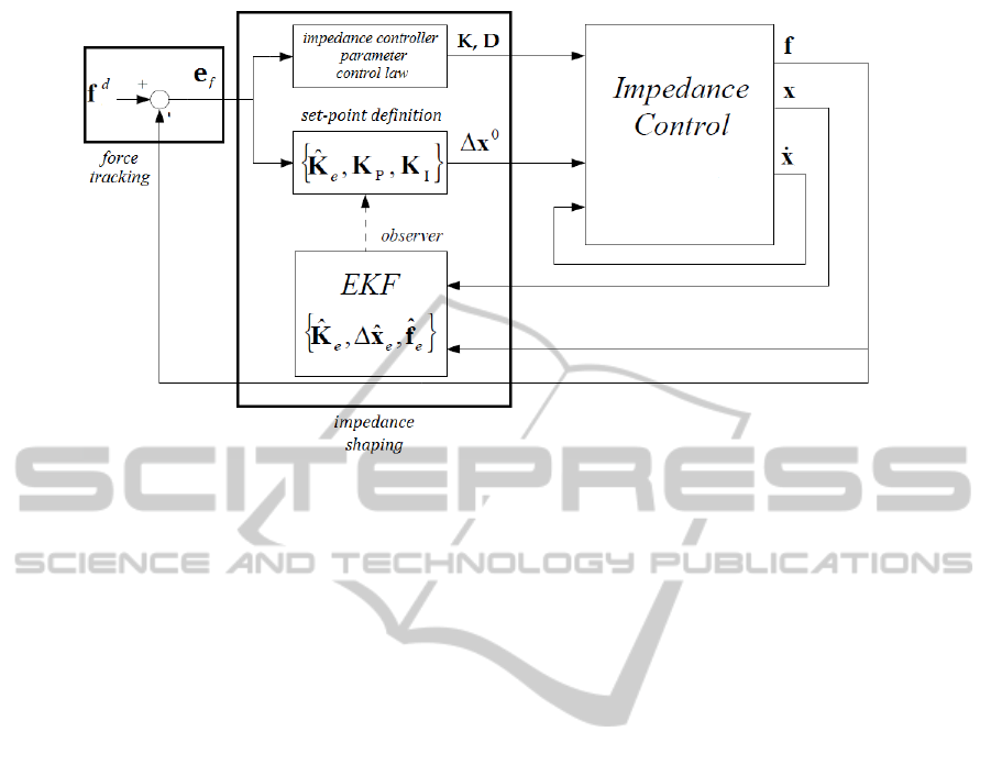
Figure 2: Impedance shaping control scheme: the set-point ∆x
0
and the stiffness and damping matrices K,D of the impedance
control are defined. An EKF is implemented to estimate the environment stiffness used in the control law.
the controlled robot at zero-force error, m
K
is the co-
efficient describing the quadratic function of the stiff-
ness matrix with respect to the force error, D is the
diagonal damping matrix of the impedance controller,
D
0
is the diagonal damping matrix of the impedance
controller at zero-force error, m
D
is the coefficient de-
scribing the quadratic function of the damping matrix
with respect to the force error, K
P
is the proportional
gain, f
e
is the force vector acting on the environment,
x
e
is the actual position of the environment and x
eq
e
is
the equilibrium position of the environment.
K
0
is set equal to 100 [N/m] and D
0
is set to have
an adimensional damping equal to 0.9 in order to have
a high compliant behavior and high damping of the
controlled robot with f
e
= 0, while m
K
> 0 and m
D
<
0 allow higher stiffness and smaller damping of the
controlled robot in order to have higher performances
with f
e
6= 0.
The main task space impedance loop is performed
by the model-based control of the manipulator at a
rate of 200 Hz, synchronously with the environment
estimation (observer in Figure 2). A model of the
multi-port robot-environment interaction is needed
to define the force setpoints in (3) through the en-
vironemt stiffness
b
K
e
, which in turn is estimated
through the deformation of the environment and the
full state of robot kinematics and exchanged forces.
Interaction states and parameters are eventually ob-
served by an EKF as described in (Roveda et al.,
2013). Signals in (1), (2) and (3) are updated to the
main KUKA LWR control loop, whose remote con-
trol mode allows the tuning of all impedance parame-
ters, together with the sampling of force and kinemat-
ics state. The remote controller is based on a real-
time Linux Xenomai platform with RTNet-patched
network interfaces.
3 COUPLED SYSTEM DYNAMICS
The dynamics of the coupled system, discussed for
stability in Section 3.2, involve a balance between the
environment and the control expressed through the
exchanged forces (described in Section 3.1).
3.1 Impedance Control and
Environment Model
As described in (Roveda et al., 2013), the dynamic
behavior of the controlled robot is equivalent to a
pure impedance system, where the stiffness K and the
damping D matrices are diagonal:
D
˙
x + K∆x = f
r
(5)
where ∆x = x − ∆x
0
is the difference between the ac-
tual robot pose and the desired one ∆x
0
as generated
in (3) and f
r
is the external interacting force/torque
vector.
Moreover, the simplest way to describe the inter-
acting environment is the linear KelvinVoigt contact
model (Fl
¨
ugge, 1975), considering a pure impedance
behavior of the interacting environment (mass M
e
-
spring K
e
- damper D
e
model):
∑
i
(M
i
e
¨
x
i
e
+ D
i
e
˙
x
i
e
+ K
i
e
∆x
i
e
) = f
e
,∀i = 1, ··,N (6)
ICINCO2014-11thInternationalConferenceonInformaticsinControl,AutomationandRobotics
446

for all the finite number N of interaction ports.
Under the hypotehsis that exchanged forces at in-
teraction ports remain unaltered by the port f
e
= f
r
= f
in (3), (4), (5) and (6).
3.2 Closed-loop Dynamics and Stability
Considering a single stable contact point, i.e. x
e
=
x, with x
eq
e
= 0, and considering a single DoF (the
impedance control decouples the DoFs of the con-
trolled robot), the coupled dynamics is therefore de-
fined using the Lagrangian approach:
T =
1
2
M
e
˙x
2
V =
1
2
K
e
x
2
+
Z
K (e
f
)(x − ∆x
0
)δx
D =
1
2
D
e
˙x
2
+
1
2
D( ˙x − ∆ ˙x
0
)
2
(7)
where T is the kinetic energy, V the potential energy
and D the dissipative energy of the coupled system.
Substituting 1, 2, 3 in 7 the potential energy becomes:
V =
1
2
K
e
x
2
+
Z
(K
0
+ m
K
e
2
f
)(−K
P
K
−1
e
e
f
)δx (8)
The dissipative energy becomes:
D =
1
2
D
e
˙x
2
+
1
2
(D
0
+ m
D
e
2
f
)(−K
P
K
−1
e
˙e
f
)
2
(9)
In order to study the coupled system stability, the ki-
netic, potential and dissipative energies have to be
written only using state variables. Therefore, the
force error e
f
can be written as follow:
e
f
= f
d
− K
e
x (10)
Substituting 10 and by applying Lagrangian approach
the dynamics of the coupled system results:
M
e
¨x = −
D
e
+ D
0
K
2
P
˙x
− m
D
( f
d
− K
e
x)
2
K
2
P
˙x − K
e
x
−
K
0
+ m
K
f
d
− K
e
x
2
(K
P
x − K
P
K
−1
e
f
d
)
(11)
In order to analyze the stability of the closed-loop sys-
tem, the positive scalar Lyapunov function candidate
is defined as:
V
Ly
= T +V (12)
The Lyapunov function candidate is therefore defined
as:
V
Ly
=
1
2
M
e
˙x
2
+
1
2
K
e
x
2
+
Z
K (x) (K
P
x − K
P
K
−1
e
f
d
)δx
(13)
Having
1
2
M
e
˙x
2
+
1
2
K
e
x
2
≥ 0 ∀ (x, ˙x), only the integral
needs to be verified:
Z
K (x) (K
P
x − K
P
K
−1
e
f
d
)δx ≥ 0 (14)
Proof. Equation (13) can be written as follow:
R
K (x) xδx
R
K (x) δx
≥
f
d
K
e
(15)
where the left side term is the baricenter of the func-
tion K (x).
Based on the quadratic function K (x) =
ax
2
+ bx + c defined in (1), the x-coordinate of
its baricenter is:
−b
2a
=
f
d
K
e
(16)
so that, substituting (16) in (15), the condition in (15)
becomes
f
d
K
e
≥
f
d
K
e
,∀(x, ˙x)
(17)
On the other hand, the time differentiation of (12)
gives:
˙
V
Ly
= M
e
˙x ¨x + K
e
x ˙x + K (x)(K
P
x − K
P
K
−1
e
f
d
) ˙x
(18)
Substituting (11) in (18), results:
˙
V
Ly
= −
D
e
+ D
0
K
2
P
˙x
2
− m
D
( f
d
− xK
e
)
2
K
2
P
˙x
2
(19)
With m
D
< 0 and m
D
defined as:
m
D
= −m
D
(20)
and imposing
˙
V
Ly
< 0, the Lyapunov conditions is:
( f
d
− xK
e
)
2
<
D
0
m
D
+
D
e
m
D
K
2
P
(21)
The closed-loop system is therefore asymptotically
stable if the quadratic force error is bounded by the
right side term of (21) . The damping quadratic func-
tion is built in order to maximize the damping term
D
0
. Moreover, it is possible to define the force refer-
ence in a way that bound the quadratic force error and
ensure the closed-loop system stability.
ImpedanceShapingControllerforRoboticApplicationsinInteractionwithCompliantEnvironments
447
4 EXPERIMENTAL TEST
The developed control strategy has been tested in
an assembly task. The set-up of the experiment is
shown in Figure 1. The experimental set-up includes
a lightweight manipulator (KUKA LWR 4+) mounted
on a rigid base and an interacting environment with
two different stiffness levels, in order to test the con-
trol strategy with different environment’s properties.
In particular, the stiffness in the vertical direction Z is
set to be soft (5000 [N/m]), while the stiffnesses in the
X and Y directions are set to be stiff (20000 [N/m]).
The impedance shaping control has been compared
with 4 different constant impedance controllers in or-
der to show its better behavior when tracking a force
reference, using the same proportional and integral
gains. In particular, for the constant impedance con-
trollers the used stiffness and damping parameters are
shown in Table 1.
In order to improve performances of the controller
an integral term is considered in the set-point ∆x
0
def-
inition:
∆x
0
= K
P
b
K
−1
e
e
f
+ K
i
b
K
−1
e
Z
e
f
(22)
4.1 Force-Tracking in Assembly Task
The assembly task (see (Roveda et al., 2013) for dis-
cussion) is performed in 5 major phases:
Phase A: Approach and contact detection in the ver-
tical direction Z.
Phase B: The on-line estimation of
b
K
e
in the vertical
direction Z starts.
Phase C: Exploration along translation components
and on-line estimation of
ˆ
K
e
. The impedance con-
trol set-point ∆x
0
and the controlled robot stiffness K
and damping D are computed as a function of force-
tracking error e
f
= f
d
task
− f (rotational components of
Table 1: The stiffness and damping parameters used in the
selected application are shown. The constant impedance
controllers parameters has been selected in order to test the
impedance control with a soft and stiff behavior and with
high and low damping.
Impedance Control Parameters
Sti f f ness[N/m] AdimensionalDamping
A shaped shaped
B 5000 0.1
C 5000 0.9
D 1000 0.1
E 1000 0.9
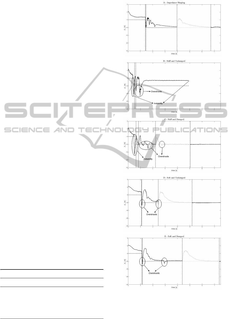
Figure 3: Desired forces (continuous lines) and measured
forces (dashed lines) in direction Z during the assembly task
for each control strategy. Phase C is highlighted in grey.
ICINCO2014-11thInternationalConferenceonInformaticsinControl,AutomationandRobotics
448
Stiffnesses during task execution
0 1 2 3 4 5 6 7
0
500
1000
1500
2000
2500
3000
3500
4000
4500
5000
[N/m]
[s]
Stiffness Z
Damping during task execution
0 1 2 3 4 5 6 7
0
0.1
0.2
0.3
0.4
0.5
0.6
0.7
0.8
0.9
1
[s]
Damping Z
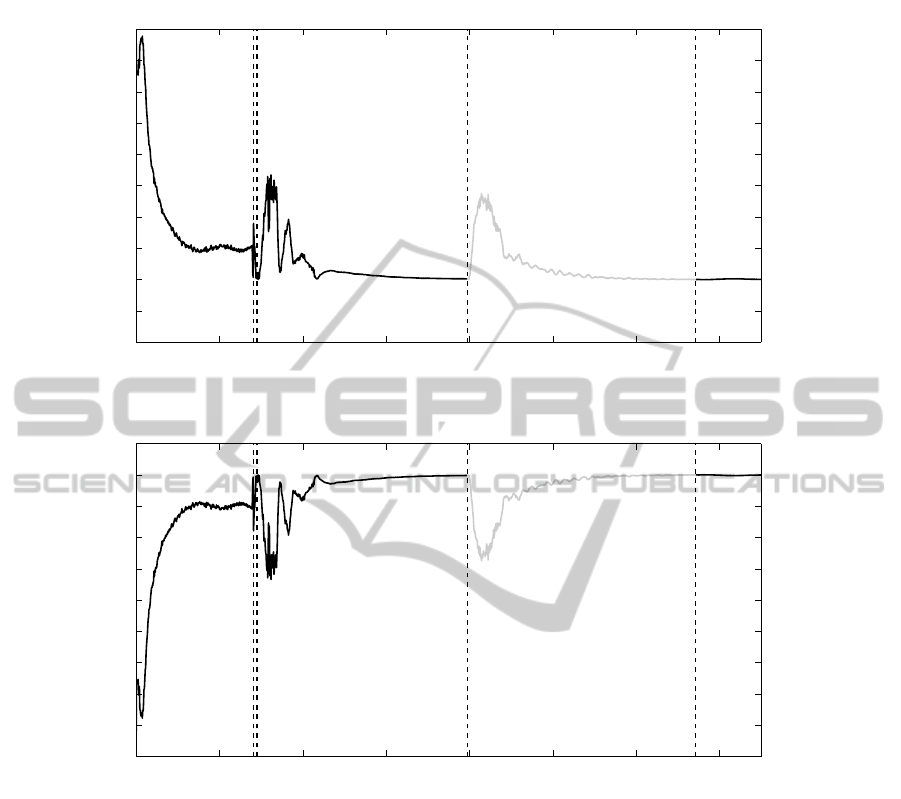
Figure 4: Impedance shaping control stiffness and damping parameters in direction Z during assembly task execution.
∆x
0
are blocked).
Phase D: Assembly proper, enabling rotations for in-
sertion and relying on
b
K
e
observed along the search-
ing directions. The set-point f
d
enables also torques.
Phase E: After tight assembly, on-line estimation
of (possibly changing)
b
K
e
.
Rotations in phase D are fastly executed to eval-
uate the capability of the control strategy to compen-
sate force overshoots using constant rotational stiff-
ness (100 [Nm/rad]) and damping parameters (0.9).
In Figure 3 the measured interaction force in direc-
tion Z is shown, highlighting different phases. Exper-
imental results show the capability of the impedance
shaping control to avoid force overshoots even dur-
ing phase D. Constant impedance controllers show
force overshoots even using high damping and a very
compliant behavior of the controlled robot. Constant
high stiffness and low damping is the worst case:
force measurements show force overshoots and unsta-
ble behaviours in the first phases of the assembly task
and the task fails during the third phase (the manip-
ulated shape escapes from the desired mounting lo-
cation). Common industrial robots are characterized
by high stiffness and low damping parameters, so this
configuration is very interesting for industrial appli-
cations.
Interaction forces in direction X and Y present the
same behaviour shown in Figure 3.
In Figure 4 stiffness K and damping D parameters
in direction Z of the impedance shaping control are
shown. Stiffness and damping parameters adapt them
self based on interaction forces.
ImpedanceShapingControllerforRoboticApplicationsinInteractionwithCompliantEnvironments
449

5 CONCLUSIONS
In this paper the impedance shaping control strategy
has been described and tested in a full rigid body as-
sembly real task with compliant support. The method
is capable to avoid force overshoots while allowing
to track a force reference using an estimate of the
environment dynamic parameters. The paper shows
the capability of the defined control strategy to satisfy
the desired requirements and compares the obtained
results to constant impedance controllers, that show
force overshoots and unstable behaviours.
Future work will extend the strategy to the rota-
tional DoFs and will investigate the optimal defini-
tion of the on-line tuning functions of the stiffness and
damping parameters and set-point gains. Moreover,
more challenging tasks will be considered (machin-
ing and surgical tasks).
ACKNOWLEDGEMENTS
This work has been partially supported by EC FP7
ACTIVE project (FP7-ICT-2009-6-270460). Opin-
ions or results expressed in this work are solely those
of the authors and do not necessarily represent those
of EC. The authors’d like to thank T. Dinon (CNR-
ITIA) for expertise, setup and experimental support.
REFERENCES
Colgate, E. and Hogan, N. (1989). An analysis of contact
instability in terms of passive physical equivalents. In
Robotics and Automation, 1989. Proceedings., 1989
IEEE International Conference on, pages 404–409.
Dubey, R. V., Chan, T. F., and Everett, S. E. (1997). Variable
damping impedance control of a bilateral telerobotic
system. Control Systems, IEEE, 17(1):37–45.
Ferraguti, F., Secchi, C., and Fantuzzi, C. (2013). A tank-
based approach to impedance control with variable
stiffness. In Proceedings of the 2013 International
Conference on Robotics and Automation (ICRA).
Fl
¨
ugge, W. (1975). Viscoelasticity. Springer New York.
Hogan, N. (1984). Impedance control: An approach to ma-
nipulation. In American Control Conference, 1984,
pages 304–313.
Ikeura, R. and Inooka, H. (1995). Variable impedance con-
trol of a robot for cooperation with a human. In
Robotics and Automation, 1995. Proceedings., 1995
IEEE International Conference on, volume 3, pages
3097–3102. IEEE.
Khatib, O. (1987). A unified approach for motion and force
control of robot manipulators: The operational space
formulation. Robotics and Automation, IEEE Journal
of, 3(1):43–53.
Lee, K. and Buss, M. (2000). Force tracking impedance
control with variable target stiffness. The Intern. Fed-
eration of Automatic Control, 16(1):6751–6756.
Mason, M. T. (1981). Compliance and force control for
computer controlled manipulators. Systems, Man and
Cybernetics, IEEE Transactions on, 11(6):418–432.
Park, J. H. and Cho, H. C. (1998). Impedance control
with varying stiffness for parallel-link manipulators.
In American Control Conference, 1998. Proceedings
of the 1998, volume 1, pages 478–482. IEEE.
Raibert, M. and Craig, J. (1981). Hybrid position/force con-
trol of manipulators. Journal of Dynamic Systems,
Measurement, and Control, 103(2):126–133.
Roveda, L., Vicentini, F., and Tosatti, L. M. (2013).
Deformation-tracking impedance control in interac-
tion with uncertain environments. In Intelligent
Robots and Systems (IROS), 2013 IEEE/RSJ Interna-
tional Conference, pages 1992–1997. IEEE.
Salisbury, J. K. (1980). Active stiffness control of a manipu-
lator in cartesian coordinates. In Decision and Control
including the Symposium on Adaptive Processes, 1980
19th IEEE Conference on, volume 19, pages 95–100.
Seraji, H. and Colbaugh, R. (1997). Force tracking in
impedance control. The International Journal of
Robotics Research, 16(1):97–117.
Villani, L., Canudas de Wit, C., and Brogliato, B. (1999).
An exponentially stable adaptive control for force and
position tracking of robot manipulators. Automatic
Control, IEEE Transactions on, 44(4):798–802.
Volpe, R. and Khosla, P. (1995). The equivalence of
second-order impedance control and proportional gain
explicit force control. The International journal of
robotics research, 14(6):574–589.
Yang, C., Ganesh, G., Haddadin, S., Parusel, S., Albu-
Schaeffer, A., and Burdet, E. (2011). Human-like
adaptation of force and impedance in stable and un-
stable interactions. Robotics, IEEE Transactions on,
27(5):918–930.
Yoshikawa, T. (1987). Dynamic hybrid position/force con-
trol of robot manipulators–description of hand con-
straints and calculation of joint driving force. Robotics
and Automation, IEEE Journal of, 3(5):386–392.
Yoshikawa, T. and Sudou, A. (1990). Dynamic hybrid po-
sition/force control of robot manipulators: On-line es-
timation of unknown constraint. In Hayward, V. and
Khatib, O., editors, Experimental Robotics I, volume
139 of Lecture Notes in Control and Information Sci-
ences, pages 116–134. Springer Berlin Heidelberg.
ICINCO2014-11thInternationalConferenceonInformaticsinControl,AutomationandRobotics
450
