
Randomized Addition of Sensitive Attributes for l-diversity
Yuichi Sei and Akihiko Ohsuga
Graduate School of Information Systems, The University of Electro-Communications, Tokyo, Japan
Keywords:
Privacy, Data mining, Anonymization.
Abstract:
When a data holder wants to share databases that contain personal attributes, individual privacy needs to be
considered. Existing anonymization techniques, such as l-diversity, remove identifiers and generalize quasi-
identifiers (QIDs) from the database to ensure that adversaries cannot specify each individual’s sensitive at-
tributes. Usually, the database is anonymized based on one-size-fits-all measures. Therefore, it is possible
that several QIDs that a data user focuses on are all generalized, and the anonymized database has no value
for the user. Moreover, if a database does not satisfy the eligibility requirement, we cannot anonymize it by
existing methods. In this paper, we propose a new technique for l-diversity, which keeps QIDs unchanged and
randomizes sensitive attributes of each individual so that data users can analyze it based on QIDs they focus
on and does not require the eligibility requirement. Through mathematical analysis and simulations, we will
prove that our proposed method for l-diversity can result in a better tradeoff between privacy and utility of the
anonymized database.
1 INTRODUCTION
In recent years, numerous organizations have begun
to provide services related to Cloud computing that
collect a great deal of personal information. This per-
sonal information can be shared with other organiza-
tions so that they can subsequently create new ser-
vices. However, the data holder should not publish
any information that identifies an individual’s sensi-
tive attributes.
A lot of research studies regarding anonymized
databases of personal information have been proposed
(e.g., (Samarati, 2001; LeFevre et al., 2008; Wu et al.,
2013)). Most of existing methods consider that the
data holder has a database of the form explicit iden-
tifiers, quasi-identifiers (QIDs), sensitive attributes,
where explicitly identifiers are attributes that explicit
identify individuals (e.g., name and phone number),
QIDs are attributesthat could be potentially combined
with public directories to identify individuals (e.g.,
zip code, age), and sensitive attributes are personal
attributes of private nature (e.g., disease) (Fung et al.,
2010).
The l-diversity technique (Machanavajjhala et al.,
2007), which enhances k-anonymity (LeFevre et al.,
2006), is one of the major anonymization techniques.
This technique removes explicit identifiers and gen-
eralizes QIDs to ensure that the adversaries cannot
specify each individual’s sensitive values with con-
fidence greater than 1/l. For example, Table 1 shows
the original patient database that a hospital wants to
publish. Consider that Name is the explicit identifier,
Sex, Age, Address, and Job are the QIDs, and Dis-
ease is the sensitive attribute. Suppose that an adver-
sary knows that Becky is included in the database and
knows Becky’s QIDs. From the database, the adver-
sary can identify Becky’s sensitive value as Sty with
100% confidence, even if we remove all the Names
from Table 1.
Table 2 shows one result of the l-diversity tech-
nique where l is set to 2. Even if the adversary
knows that Becky is included in Table 2 and knows
Becky’s QIDs, he cannot know whether Fever or Sty
is Becky’s disease. That is, he cannot identify Becky’s
sensitive value with greater than 50% (=1/2) confi-
dence. Table 3 is another result of the l-diversity tech-
nique. If Tables 2 and 3 are both published, the adver-
sary can identify Becky’s disease as Sty with 100%
confidence, so the data holder usually anonymizes Ta-
ble 1 once and publishes the anonymized table (i.e.,
either Table 2 or Table 3 only) to the all data users.
Therefore, the data holder should anonymize the
database based on one-size-fits-all measures. Sup-
pose that two data users, A and B, receive Table 2, and
suppose that data user A wants to know the difference
between male and female, while data user B wants to
350
Sei Y. and Ohsuga A..
Randomized Addition of Sensitive Attributes for l-diversity.
DOI: 10.5220/0005058203500360
In Proceedings of the 11th International Conference on Security and Cryptography (SECRYPT-2014), pages 350-360
ISBN: 978-989-758-045-1
Copyright
c
2014 SCITEPRESS (Science and Technology Publications, Lda.)

Table 1: Patient table.
Name
Sex Age Address Job Disease
Alex M 41 13000 Artist Fever
Becky
F 41 17025 Artist Sty
Carl
M 50 13021 Writer Cancer
Diana
F 51 14053 Nurse HIV
Edward
M 68 15000 Writer Chill
Flora
F 69 16022 Nurse HIV
Greg
M 72 13001 Artist Cut
Hanna
F 77 17001 Artist Cancer
Table 2: 2-diversity by existing method.
Sex
Age Address Job Disease
* 41 13*-17* Artist Fever
*
41 13*-17* Artist Sty
*
50-51 13*-14* * Cancer
*
50-51 13*-14* * HIV
*
68-69 15*-16* * Chill
*
68-69 15*-16* * HIV
*
72-77 13*-17* Artist Cut
*
72-77 13*-17* Artist Cancer
Table 3: 2-diversity by existing method (2).
Sex
Age Address Job Disease
M 41-72 13* Artist Fever
F
41-77 17* Artist Sty
M
50-68 13*-15* Writer Cancer
F
51-69 14*-16* Nurse HIV
M
50-68 13*-15* Writer Chill
F
51-69 14*-16* Nurse HIV
M
41-72 13* Artist Cut
F
41-77 17* Artist Cancer
Table 4: 2-diversity by proposed method.
Sex
Age Address Job Disease
M 41 13000 Artist {Fever, Flu}
F
41 17025 Artist {Fever, Sty}
M
50 13021 Writer {Cold, Cancer}
F
51 14053 Nurse {HIV, Pus}
M
68 15000 Writer {Chill, Cut}
F
69 16022 Nurse {Cold, HIV}
M
72 13001 Artist {Cut, Fever}
F
77 17001 Artist {Cancer, Flu}
know the differences among age. Although data user
B may know the differences among age from Table
2, data user A cannot know any differences between
sexes because the values of sex are all generalized.
On the other hand, suppose that data users A and B
receive Table 3 rather than Table 2. In this case, data
user A can analyze Table 3, but data user B cannot an-
alyze it effectively because ages are too generalized.
In this paper, we deal with this specific problem.
Our proposed method keeps QIDs unchanged and
adds l − 1 dummy values into sensitive attributes in
order to satisfy l-diversity. The resulting anonymized
database is shown in Table 4. Because all QIDs
are not changed, all data users can analyze the
anonymized database in theirpreferred ways. We pro-
pose a protocol that estimates the original data dis-
tribution of sensitive values according to each data
user’s preferred QIDs from the anonymized database,
as well as an anonymization protocol for the data
holder. If the number of records in the table is large,
data users can analyze it with a high degree of accu-
racy by the proposed method.
It is worth noting that we need not protect QIDs
when we use k-anonymity or l-diversity as pri-
vacy models. Although QIDs of databases may be
anonymized as a result of anonymization, most of ma-
jor privacy models such as k-anonymity, l-diversity
and t-closeness offer no guarantee of anonymizing
QIDs because their aims are not to protect QIDs but
to protect sensitive attributes.
Moreover, one major limitation of existing tech-
niques for l-diversity is the eligibility requirement,
which requires that “at most |T|/l records of T carry
the same sensitive value” where |T| represents the
number of records of an original database T (Xiao
et al., 2010). Our proposed method does not require
the eligibility requirement, therefore our method can
be applied to any databases when l is less than the
number of distinct sensitive values.
The rest of this paper is organized as follows. Sec-
tion 2 presents the models of applications and attacks.
Section 3 defines privacy and utility as used in this
paper. Section 4 discusses the related methods. Sec-
tion 5 presents the design of our algorithm. The re-
sults of a mathematical analysis and our simulations
are presented in Section 6, and Section 7 concludes
the paper.
2 ASSUMPTIONS
2.1 Application Model
A data holder has a database that contains personal in-
formation. Such information consists of explicit iden-
tifiers, QIDs, and sensitive attributes as described in
Section 1. The database can contain non-sensitive at-
tributes that are not explicit identifiers, QIDs, or sen-
sitive attributes. We can publish these non-sensitive
attributes without them being anonymized if they are
important for data analysis.
We assume that the data holder wants to publish
the database for collaborating with data users. Be-
RandomizedAdditionofSensitiveAttributesforl-diversity
351

Table 5: l-diversity does not protect any values of QIDs
when the original database satisfies l-diversity (here, l=2).
Sex
Age Address Job Disease
M 31 13000 Artist Fever
M
31 13000 Artist Sty
M
52 13021 Writer Cancer
M
52 13021 Writer HIV
cause of privacy concerns, the data holder wants to
anonymize the database in order to ensure that any
adversaries cannot identify each individual’s sensitive
attribute.
In this paper,we assume that the data user wants to
know what kinds of people tend to have certain sensi-
tive values. As a result, we might find that older men
are more likely to get lung cancer than young women
if the anonymized table contains age and sex as QIDs
(or non-sensitive attributes) and disease as a sensitive
attribute.
We assume that we must protect sensitive at-
tributes, but we do not need to protect QIDs. This
assumption is widely accepted in research studies re-
lated to k-anonymity, l-diversity, and so on. If there
are l records that have the same values of QIDs,
these records are not anonymized in any methods
for l-diversity. For example, if a data holder want
to anonymize Table 5, the values of QIDs are not
anonymized at all when l=2.
If we want to protect some of the QIDs, then we
can treat them as sensitive attributes.
2.2 Attack Model
We assume that the data holder is an honest entity, but
the data users may be malicious entities. Moreover,
we assume that the data users may collude with each
other to identify each individual’s sensitive attributes.
3 NOTATIONS AND
MEASUREMENTS
3.1 Notations
Let T and T
∗
denote the original and anonymized
database respectively. Let N denote the number of
records of T or T
∗
and let r
i
and r
∗
i
denote the i-th
record of T and T
∗
, respectively.
S represents the domain of possible sensitive at-
tributes that can appear in the database and s
i
means
the i-th value of S (i = 0, .. .,|S| −1). Let Q be the set
of QIDs that a data user wants to analyze and let Q(i)
be the i-th QID of Q (i = 0,...,|Q| − 1).
Let Q(i) denote the domain of possible values that
can appear in Q(i) and let q(i)
j
denote the j-th value
of Q(i).
For example, S is {Fever, Sty, ...} in Table 1. Q
is {Sex}, Q(0) is Sex, Q(0) is {M, F} and q(0)
0
is
M and q(0)
1
is F if a data user wants to know the
difference between the sexes (male and female). In
this case, the data user might find that people who are
men have the highest risk of getting cancer.
For another example, if the data user wants to an-
alyze sensitive attributes based on the combination of
sexes and categories of age ([0-9], [10-19], ..., [90-
99]), Q is {Sex, Age}, Q(0) is {M, F} and Q(1) is
{[0-9], .. ., [90-99]}. In this case, the data user might
find that men ages between 30-39 have the highest
risk of getting cancer.
The value of a sensitive attribute of a record r
is represented by E(r). For example, E(r
0
) returns
Fever in Table 1. In a similar way, E(r
∗
0
) returns
{Fever, Flu} in Table 4.
Let C denote all the combinations of the elements
of Q(0),...,Q(|Q| − 1):
C = Q(0) × Q(1) × ...× Q(|Q| − 1). (1)
Let c
i
denote the i-th element of C (i = 0,...,|C| −
1). For example, if the data user wants to analyze
sensitive attributes based on sexes and categories of
age ([0-9], .. ., [90-99]), c
0
is (M, [0-9]), c
1
is (M,
[10-19]), . . ., c
|C|−1
is (F, [90-99]).
3.2 Measurement of Privacy
Many existing papers use l-diversity as a privacymea-
surement (Machanavajjhala et al., 2007; Xiao et al.,
2010; Cheong, 2012). Althoughthere are several vari-
ations of l-diversity, we use a simple interpretation.
Definition 1 (QID group): We denote a set of
records that has same values of all QIDs as a QID
group.
For example, the first and second records in Table
2 are a QID group because their values of QIDs are
the same (*, 41, 13*-17*, Artist).
Definition 2 (l-diversity): The anonymized ta-
ble T
∗
satisfies l-diversity if the relative frequency of
each of the sensitive values does not exceed 1/l for
each QID group of T
∗
.
This definition of l-diversity is also widely used,
such as in the cases of (Kenig and Tassa, 2011; Xiao
and Tao, 2006; Nergiz et al., 2013).
For example, all QID groups of Tables 2 and 3
have 2 records and 2 distinct sensitive values. There-
fore, these tables satisfy 2-diversity. Then, see Ta-
ble 4. Each QID group has only one record, but each
record has 2 distinct sensitive values. We consider
Table 4 also satisfies 2-diversity in this paper.
SECRYPT2014-InternationalConferenceonSecurityandCryptography
352

3.3 Measurement of Utility
A data user estimates the distribution of sensitive at-
tributes for each c
i
(i = 0,...,|C| − 1) as described in
Section 2. Let V
i, j
denote the number of records that
are categorized to c
i
according to their QIDs and have
a sensitive attribute s
j
in the original table. Also, let
c
V
i, j
denote the estimated number of values of V
i, j
for
the data user.
Let N
i
denote the number of records that are cat-
egorized to c
i
according to their QIDs. We can use
the Mean Squared Errors (MSE) between
c
V
i, j
/N
i
and
V
i, j
/N
i
to quantify the utility for category c
i
:
σ
2
(i) =
1
|S|
|S|−1
∑
j=0
(
V
i, j
N
i
−
c
V
i, j
N
i
)
2
(2)
This utility measurement is widely used in many
studies (Xie et al., 2011; Huang and Du, 2008; Groat
et al., 2012).
4 RELATED WORK
Many algorithms for k-anonymity have been pro-
posed. The basic definition of k-anonymity is as fol-
lows:
If one record in the table has some value QID,
at least k − 1 other records also have the value QID
(Fung et al., 2010).
Due to the fact that finding an optimal k-
anonymity is NP-hard (Meyerson and Williams,
2004), many existing algorithms for k-anonymity
search for better anonymization through heuristic ap-
proaches.
Datafly (Sweeney, 2002) is a bottom-up greedy
approach and it generalizes QIDs until all combi-
nations of QIDs appear at least k times. Mondrian
(LeFevre et al., 2006), which is an efficient top-down
greedy approach, is widely used in many other studies
as a base method.
Although k-anonymity can protect individual
identities, there are times when it cannot protect indi-
viduals’ sensitive attributes. For example, the fourth
and sixth rows in Table 3 are an equivalence class be-
cause their QIDs are all the same (F, 51-69, 14*-16*,
Nurse). Suppose that an adversary knows Diana’s
QIDs and she is included in Table 3. The adversary
cannot identify which row of the fourth and sixth rows
is Diana’s, but the adversary can identify Diana’s sen-
sitive attribute is HIV because the sensitive attributes
of both the rows are HIV.
l-diversity (Machanavajjhala et al., 2007) ensures
that the probability of identifying an individual’s sen-
sitive attribute is less than or equal to 1/l. There
are many research studies related to l-diversity (e.g.,
(Kabir et al., 2010; Cheong, 2012)).
Although many algorithms for k-anonymity or l-
diversity other than the research studies previously
mentioned havebeen proposed, most of all algorithms
keep sensitive attributes unchanged and generalize
QIDs. Changing QIDs leads to the problems men-
tioned in Section 1.
If all data users analyze the anonymized table in
the same way or if we believethat all data users do not
collude with each other for identifying an individual’s
sensitive attributes, then we can use workload-aware
anonymization techniques (LeFevre et al., 2008).
However, in the situation described in Section 2, we
need other anonymization techniques that do not rely
on those assumptions.
Xiao et al. (Xiao and Tao, 2006) and Sun et al.
(Sun et al., 2009) proposed an algorithm based the
Anatomy technique. Their algorithms publish two ta-
bles; one is a non-sensitive table that contains QIDs
without change and the other is a sensitive table.
By joining of the two tables, data users can analyze
them. Because the resulting table have many dummy
records (e.g., several times of the number of original
records), such anonymized data may become useless
for data analysis.
TP (Xiao et al., 2010) is the algorithm with
a non-trivial bound on information loss. The au-
thors compared TP with other techniques for l-
diversity (single-dimensional generalization method
TDS (Fung and Yu, 2005) and multi-dimensionalgen-
eralization method Hilbert (Ghinita, 2007)) and they
proved that TP outperforms these single- or multi-
dimensional methods.
We compare Anatomy and TP with our proposed
method in Section 6.
To the best of our knowledge, all existing tech-
niques for l-diversity requires the eligibility require-
ment as described in Section 1. Therefore, if
more than |T|/l records of original database T have
the same sensitive value, we cannot anonymize the
database.
The privacy measure of t-closeness (Li et al.,
2007) is stronger than l-diversity. It requires that the
distribution of sensitive values in each set of records
that have the same QID values should be close to the
distribution of the whole database.
Differential privacy (Dwork, 2006; Domingo-
Ferrer, 2013) makes user data anonymous by adding
noise to a dataset so that an attacker cannot deter-
mine whether or not a particular point of user data
is included. Although differential privacy represents
one of the strongest privacy models (Nikolov et al.,
2013), the data holder cannot publish the anonymized
RandomizedAdditionofSensitiveAttributesforl-diversity
353

database. The data holder should manage the original
database and respond to each data user’s query every
time. Therefore, the data holder’s cost is high, data
users cannot analyze the anonymized database freely,
and it is vulnerable to malicious intrusion (Clifton and
Anandan, 2013). In this paper, we assume that we
need anonymization techniques other than differential
privacy because of these limitations.
5 PROPOSAL
Our proposed method consists of two steps; random-
ization for the data holder and reconstruction for the
data user.
For the data holder, we generate and add l − 1 val-
ues randomly for a sensitive attribute of each record
in the original database.
For the data user, the user first determines which
QIDs should be analyzed in terms of the relationships
between the QIDs and the sensitive attributes. Then,
the number of records is estimated in each combina-
tion of the QIDs and the sensitive attribute. For exam-
ple, suppose that the domain of the sensitive attribute
contains HIV, Fever, and Cancer. Also, suppose that
the data user wants to analyze the difference between
male and female. In this case, we should estimate
each number of records in which a sensitive attribute
is HIV, Fever, and Cancer, and where Sex is Male and
Female, respectively.
5.1 Anonymization Protocol
We generate and add distinct l − 1 values randomly
for a sensitive attribute of each record in the original
database for the data holder. Algorithm 1 shows the
anonymization protocol.
The function rand(S) returns an element of S ran-
domly. The data holder executes Algorithm 1 for each
record.
THEOREM 5.1. Algorithm 1 can always generate
l-diversity Table T
∗
from an original Table T if |S| is
larger than or equal to l.
Proof. After conducting Algorithm 1 for Table T,
the algorithm generates an anonymized Table T
∗
in
which each record has l distinct sensitive values. Sup-
pose that a QID group has δ (δ = 1,...,N) records of
T
∗
. The possible maximum number of occurrences of
each sensitive value within the δ records is δ because
each sensitive value does not appear more than once
in a record. On the other hand, the total number of
sensitive values in the QID group is δ × l if we use
Algorithm 1: Anonymization protocol for record r.
Input: Domain of a sensitive attribute S, Privacy
level l
Output: Set of anonymized sensitive values for
record r
1: Creates empty set R
2: R ⇐ R∪ {E(r)}
/*Generates and adds dummy sensitive at-
tributes*/
3: while |R| < l do
4: R ⇐ R ∪ {rand(S)}
5: end while
6: return R
Algorithm 1 because each record has l sensitive val-
ues, thus, the possible maximum relative frequency
of each of the sensitive values in the QID group is
1/l.
5.2 Estimation Protocol
The data user who received the anonymized table es-
timates the distribution of sensitive attributes for each
c
i
(i = 0,... , |C| − 1). We use V
i, j
to represent the ac-
tual number of records, which are categorized to c
i
and have a sensitive attribute s
j
. Let
c
V
i, j
denote the
estimated V
i, j
.
First, the data user counts how many records that
are categorized c
i
occur in the anonymized database,
that is,
N
i
=
N−1
∑
h=0
G(r
∗
h
,c
i
), where G(r
∗
,c) =
(
1 (r
∗′
s QIDs are categorized to c)
0 (otherwise)
(3)
In a similar way, the data user counts how many
records that are categorized to c
i
and have a set of
sensitive attributes that contain s
j
in the anonymized
database:
W
i, j
=
N−1
∑
h=0
H(r
∗
h
,c
i
,s
j
),where H(r
∗
,c, s) =
(
1 (r
∗′
s QIDs are categorized to c and s ∈ E(r
∗
))
0 (otherwise)
(4)
If a record r has s
j
as its original sensitive at-
tribute, then s
j
is included in E(r
∗
) with probability
1 and s
j
2
s.t., j 6= j
2
is included in E(r
∗
) with proba-
bility
P
E
=
l − 1
|S| − 1
. (5)
SECRYPT2014-InternationalConferenceonSecurityandCryptography
354

Let the
d
W
i, j
be the maximum likelihood estimate
of W
i, j
. Then, we have
d
W
i, j
= N
i
−
∑
j
2
6= j
(1− P
E
)
d
V
i, j
2
. (6)
The data user constructs a linear system of equa-
tions in |S| variables of
c
V
i, j
( j = 0,... , |S| − 1) from
Equation 6 for each c
i
. Here, we set the value of W
i, j
calculated from T
∗
by Equation 4 to
d
W
i, j
in Equa-
tion 6. By solving the linear system of equations,
the data user gets
c
V
i, j
for each i = 0,...,|C| − 1 and
j = 0,...,|S| − 1. Each value of
c
V
i, j
is an unbiased
maximum likelihood estimate of V
i, j
.
We show this estimation protocol in Algorithm 2.
A data user executes this algorithm for each c
i
(i =
0,...,|C| − 1) based on his own C.
Algorithm 2: Server protocol for c
i
.
Input: Anonymized database T
∗
, Domain of a sensi-
tive attribute S
Output: Distribution of sensitive attributes in c
i
1: Creates Array W,
b
V
/*Calculates N
i
*/
2: N
i
⇐ result calculated by Eq. 3
/*Calculates each W
i, j
*/
3: for j = 0, ...,|S| − 1 do
4: W
i, j
⇐ result calculated by Eq. 4
5: end for
/*Calculates P
E
*/
6: P
E
⇐ result calculated by Eq. 5
/*Creates and solves the linear system of equa-
tions*/
7: Creates Eq. 6 for all j = 0,... , |S| − 1
8: for j = 0, ...,|S| − 1 do
9:
c
V
i, j
⇐ each result calculated by the linear sys-
tem of equations
10: end for
11: return
c
V
i, j
( j = 0,...,|S| − 1)
5.3 Expectation of MSE
The data user should understand the expectation of the
MSE between the estimated distribution and the origi-
nal distribution of sensitive attributes in each category
c
i
(i = 0, . . . ,|C| − 1) for valuable data analysis. We
propose the calculation method even if the data user
does not have the original database.
From Equation 2, the expected value of MSE for
a category c
i
, i.e., E[σ
2
], is calculated by
E[σ
2
] =
1
|S|
|S|−1
∑
j=0
E
"
(
V
i, j
N
i
−
c
V
i, j
N
i
)
2
#
(7)
Because
c
V
i, j
is the unbiased estimator of V
i, j
, we
have E[
c
V
i, j
] = V
i, j
. Therefore, E[(V
i, j
−
c
V
i, j
)
2
] repre-
sents the variance of
c
V
i, j
. LetVar(
c
V
i, j
) be the variance
c
V
i, j
. The expected value of σ
2
is calculated by
E[σ
2
] =
1
N
2
i
1
|S|
|S|−1
∑
j=0
Var(
c
V
i, j
). (8)
The simultaneous equations created by Equation
6 for all j are the same as the following equation by
deformation.
M ·
~
V
τ
=
~
W
τ
,
where M =
0 1− P
E
··· 1− P
E
1− P
E
0 ··· 1− P
E
.
.
.
.
.
.
.
.
.
.
.
.
1−P
E
1−P
E
··· 0
,
~
V = (
c
V
i,0
,
c
V
i,1
,...,
\
V
i,|S|−1
),
~
W = (N
i
−W
i,0
,N
i
−W
i,1
,...,N
i
−W
i,|S|−1
).
(9)
Therefore, we have
~
V
τ
= M
−1
·
~
W
τ
. (10)
In general, if X and Y are random variables and a
and b are constant, then we have
Var(aX + bY) = a
2
Var(X) + b
2
Var(Y) + 2abCov(X,Y ),
(11)
where Cov(X,Y) represents the covariance be-
tween X and Y. Let M
−1
j
1
, j
2
denote the j
1
-th row and
j
2
-th column element of the inverse matrix of M.
Because we have
d
V
i, j
1
=
∑
j
2
M
−1
j
1
, j
2
(N
i
− W
i, j
2
) from
Equation 10, we get from Equation 11,
Var(
d
V
i, j
1
) =
∑
j
2
(M
−1
j
1
, j
2
)
2
Var(N
i
−W
i, j
2
)
+
∑
j
2
, j
3
( j
2
6= j
3
)
M
−1
j
1
, j
2
M
−1
j
1
, j
3
Cov(N
i
−W
i, j
2
,N
i
−W
i, j
3
).
(12)
Let P
j
denote the probability that an arbitrary E(r
∗
)
contains s
j
, let P
j
2
, j
3
denote the probability that it con-
tains s
j
2
and s
j
3
, let P
j
2
,
j
3
denote the probability that
it contains s
j
2
but does not contain s
j
3
, and let P
j
2
, j
3
denote the probability that it contains s
j
3
but does not
RandomizedAdditionofSensitiveAttributesforl-diversity
355

contain s
j
2
. We get
Var(N
i
−W
i, j
2
) = E[W
2
i, j
2
] − E[W
i, j
2
]
2
=
N
i
∑
h=0
P
h
j
2
(1− P
j
2
)
N
i
−h
N
i
C
h
· h
2
− (NP
j
2
)
2
= N
i
P
j
2
(1− P
j
2
),
Cov(N
i
−W
i, j
2
,N
i
−W
i, j
3
) =
E[W
i, j
2
W
i, j
3
] − E[W
i, j
2
]E[W
i, j
3
]
=
N
i
∑
h=0
N
i
−h
∑
t=0
N
i
−h−t
∑
u=0
h
P
h
j
2
, j
3
P
t
j
2
,
j
3
P
u
j
2
, j
3
· (1− P
j
2
, j
3
− P
j
2
,
j
3
− P
j
2
, j
3
)
N
i
−h−t−u
·
N
i
C
h
·
N
i
−h
C
t
·
N
i
−h−t
C
u
· (h+ t)(h+ u)
i
− N
i
P
j
2
N
i
P
j
3
= N
i
(P
j
2
, j
3
+ (P
j
2
, j
3
+ P
j
2
,
j
3
)(P
j
2
, j
3
+ P
j
2
, j
3
)(N
i
− 1))
− N
i
P
j
2
N
i
P
j
3
(13)
If we assume that each P
j
is the same and it is
independent of each other, we get
P
j
2
= P
j
3
=
l
|S|
P
j
2
, j
3
=
l
|S|
·
l − 1
|S| − 1
P
j
2
,
j
3
= P
j
2
, j
3
=
l
|S|
· (1−
l − 1
|S| − 1
)
(14)
We get from Equations 8, 12, 13 and 14
E[σ
2
] =
1
N
i
"
l
|S|
(1−
l
|S|
)
∑
j
2
(M
−1
j
1
, j
2
)
2
−
l(|S|− l)
(|S| − 1)|S|
2
·
∑
j
2
, j
3
, j
2
6= j
3
M
−1
j
1
, j
2
M
−1
j
1
, j
3
#
.
(15)
The inverse matrix of M is represented by
M
−1
=
1
|S|−l
2−|S| 1 . . .
1 2−|S| ...
.
.
.
.
.
.
.
.
.
. (16)
Therefore, we get
∑
j
2
(M
−1
j
1
, j
2
)
2
=
1
|S|−l
2
(2−|S|)
2
+ |S| −1
,
(17)
and
∑
j
2
, j
3
, j
2
6= j
3
M
−1
j
1
, j
2
M
−1
j
1
, j
3
=
1
|S|−l
2
· {2(2−|S|)(|S| − 1) + (|S| − 1)(|S| − 2)}
.
(18)
As a result, from equations 15, 17, and 18, we get
the expected MSE between the original and estimated
distributions of sensitive attributes in c
i
;
E[σ
2
]=
l(|S| − 1)
2
N
i
(|S| − l)|S|
2
. (19)
5.4 Analysis
5.4.1 Prerequisite for Anonymization
Our proposed method does not require the eligibility
requirement because our method does not generalize
any QIDs nor insert dummy records. Let |S| denote
the number of kinds of sensitive values. If l ≤ |S|, we
can anonymize any databases for l-diversity because
we can add l− 1 sensitive values to each user’s sensi-
tive attribute. Note that setting l > |S| is meaningless
in terms of the definition of l-diversity.
5.4.2 Cost Analysis
The time complexity of the anonymization protocol at
the data holder is O(l). This protocol is computation-
ally simple as we know from Algorithm 1.
Solving the linear system of equations with |S| di-
mensions is the most expensive step in the estima-
tion protocol. We can solve a linear system of equa-
tions by solving a |S| × |S| matrix equation. The time
complexity of solving a |S| × |S| matrix equation is
O(g|S|
2
), where g is a parameter of the number of re-
cursive iterations if we use the Gauss-Seidel method.
Since we solved the linear system of equations for
each category c, the resulting time complexity is rep-
resented by O(g|S|
2
|C|).
6 EVALUATION
6.1 Mathematical Analysis and
Simulations of Synthetic Data
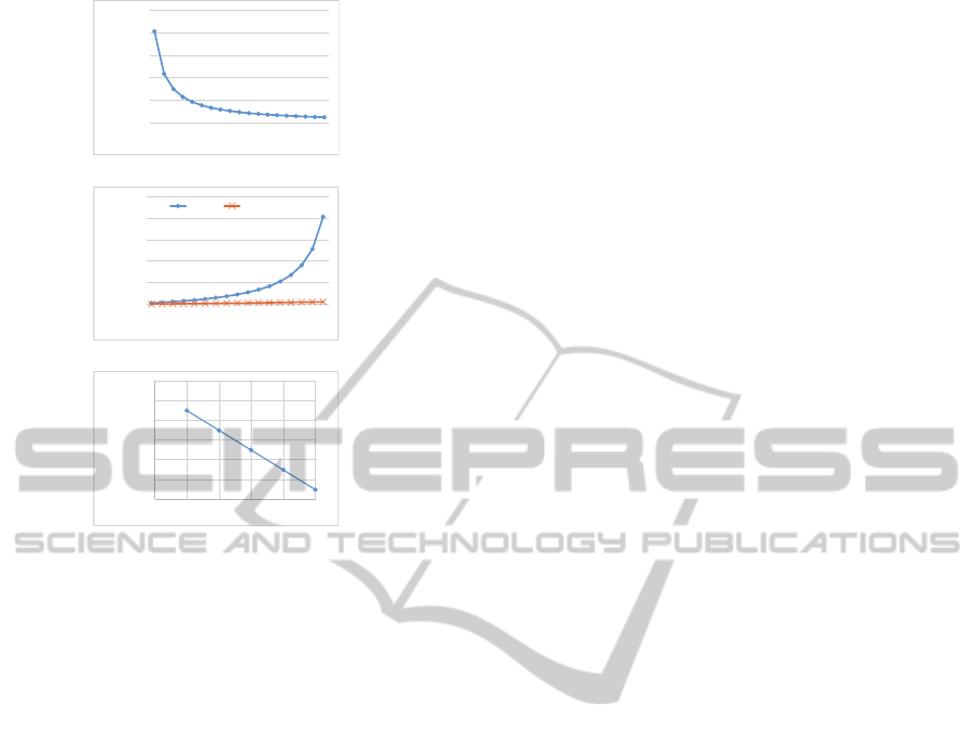
Figure 1 shows the results of mathematical analysis.
We assume that we have N records categorized to c
that are one of the combinations of elements of QIDs
that a data user wants to analyze. In this subsection,
we calculate MSE by Equation 2 between the distri-
bution of original sensitive attributes and those of es-
timated sensitive attributes in the category c.
In the first evaluation, we set the number of
records N to 1,000 and l to 5. Figure 1(a) represents
the results of the MSE. We know from Fig. 1(a) that
the MSE tends to be decreasing with an increase of
|S|.
SECRYPT2014-InternationalConferenceonSecurityandCryptography
356
0
0.0002
0.0004
0.0006
0.0008
0.001
10 20 30 40 50 60 70 80 90 100
MSE
|S|
(a) MSE vs. |S|
0
0.002
0.004
0.006
0.008
0.01
2 4 6 8 10 12 14 16 18
MSE
l
|S|=20 |S|=100
(b) MSE vs. l
0.000001
0.00001
0.0001
0.001
0.01
0.1
1
1 10 100 1000 10000100000
MSE
N
(c) MSE vs. N
Figure 1: Results of mathematical analysis.
Then, we calculate the MSE by changing the pri-
vacy level l. The results are shown in Fig. 1(b). We
changed l from 2 to 18 based on the settings of many
existing studies (Yao et al., 2012; Nergiz et al., 2013;
Hu et al., 2010). In this evaluation, we set the num-
ber of records N to 1,000 and the number of possible
sensitive attributes |S| to 20 and 100. From the fig-
ure, we know that the MSE of our proposed method
increases by increasing l. If we set l to near |S|,
the MSE increases exponentially, although the MSE
keeps a small value if l is much less than |S|. Never-
theless, we show that our proposed method can result
in a small MSE even if we set l to very near |S| (i.e.,
|S| − 1) by simulations of a real data set in the next
subsection.
Next, we conducted an experiment to analyze the
effects of changing the number of records N. Figure
1(c) shows the results of this. In this evaluation, we
set l to 5 and |S| to 20. We know that the MSE reduced
relative to N.
Finally, we conducted simulations by setting pa-
rameters (|S|, l, and N) to the same values in the math-
ematical analysis described above. The underlying
distributions of sensitive attributes were set to Uni-
form distribution, Gaussian distribution, and Poisson
distribution. In all simulations, the results are almost
the same as that of the mathematical analysis.
6.2 Real Data Set Evaluation Results
We evaluated the MSE by using real data sets, which
are OCC, SAL and Adult. OCC and SAL are obtained
from (Minnesota Population Center, ). Many existing
studies such as (Xiao et al., 2010) and (Xiao and Tao,
2006) use this data sets. OCC has an attribute Occu-
pation as a sensitive attribute and has attributes Age,
Gender, Marital Status, Race, Birth Place, Education,
Work Class as QIDs. SAL has an attribute Income
as a sensitive attribute and has the same QIDs as in
OCC. The number of distinct values of each attribute
is shown in Table 6.
We create 7 sets of database, OCC-1, OCC-2, ...,
OCC-7 from OCC. Each database OCC-d has the first
d QIDs in Table 6 and a sensitive attribute Occupa-
tion. For example, OCC-3 has Age, Gender, Mari-
tal Status as QIDs and Occupation as a sensitive at-
tribute. Similarly, we also create 7 sets of database
SAL-d (d = 1,...,7) from SAL.
The Adult data set consists of 15 attributes (e.g.,
Age, Sex, Race, Relationship shown in Table 7) and
has 45,222 records after the records with unknown
values are eliminated. Adult data set (UCI Machine
Learning Repository, ) used in many studies on pri-
vacy (Machanavajjhala et al., 2007; Sun et al., 2009).
Wet create 15 sets of database, Adult(1), Adult(2), . ..,
Adult(15)from Adult. Each database Adult(d)has the
d’th attribute in Table 7 as a sensitive attribute and has
other attributes as QIDs. For example, Adult-2 has
Work Class as a sensitive attribute and has Age, Final
Weight, Education, ... as QIDs.
Following (Xiao and Tao, 2006), we consider
a query involves qd random QIDs A
1
,...,A
qd
, and
the sensitive attribute, where qd represents the query
dimensionality parameter. For example, when the
database is SAL-4 and qd=3, {A
1
, A
2
, A
3
} is a ran-
dom 3 sized subset of {Age, Gender, Marital Status,
Race}. We assume that data users want to know the
number of persons whose attribute A
i
(i = 1,...,qd) is
the specific value. Therefore, we create random val-
ues for each A
i
as the specific values in each query.
Let b
i
denote the size of the random values for at-
tribute A
i
. Following (Xiao and Tao, 2006), the value
of b
i
is calculated by the expected query selectivity s:
b
i
= ⌈|A
i
| · s
1/(qd+1)
⌉ (20)
where |A
i
| represents the number of distinct values of
A
i
in the original database.
We compared our method with Anatomy and TP,
which were described in Section 4. All experiments
were conducted on an Intel Xeon CPU E5-2687W v2
@ 3.40GHz 3.40GHz personal computer with 12 GB
of RAM.
RandomizedAdditionofSensitiveAttributesforl-diversity
357

0.00E+00
5.00E-05
1.00E-04
1 2
MSE
qd
Proposal TP Anatomy
(a) OCC-3
0.00E+00
2.00E-05
4.00E-05
1 2
MSE
qd
Proposal TP Anatomy
(b) SAL-3
0.00E+00
2.00E-05
4.00E-05
6.00E-05
8.00E-05
1 2 3 4
MSE
qd
Proposal TP Anatomy
(c) OCC-5
0.00E+00
1.00E-05
2.00E-05
3.00E-05
1 2 3 4
MSE
qd
Proposal TP Anatomy
(d) SAL-5
0.00E+00
1.00E-04
2.00E-04
3.00E-04
4.00E-04
1 2 3 4 5 6
MSE
qd
Proposal TP Anatomy
(e) OCC-7
0.00E+00
5.00E-05
1.00E-04
1.50E-04
2.00E-04
1 2 3 4 5 6
MSE
qd
Proposal TP Anatomy
(f) SAL-7
Figure 2: MSE vs. query dimensionality qd.
0.00E+00
1.00E-05
2.00E-05
3.00E-05
4.00E-05
5 10 15
MSE
l
Proposal TP Anatomy
(a) OCC-5
0.00E+00
2.00E-05
4.00E-05
6.00E-05
5 10 15
MSE
l
Proposal TP Anatomy
(b) SAL-5
Figure 3: MSE vs. l.
We set l to 10, s to 0.07, and qd to 3 as a default
value. In each simulation, we generated 1,000random
queries based on qd and Equation 20, and calculate
MSEs based on Equation 2.
In the first simulation with OCC and SAL, we con-
ducted an analysis to determine how the number of
QIDs and qd affect the MSE. We changed the number
of QIDs d from 3 to 7 and changed qd from 1 to d −1.
Figure 2 shows the results. Figures 2(a), 2(c) and 2(e)
are the results of OCC, and Figs. 2(b), 2(d) and 2(f)
are the results of SAL. When the number of QIDs d
is 3, the MSEs of our proposed method and TP are
almost the same. On the other hand, in the results of
other settings, the MSEs of our proposed method is
much fewer than other methods.
In the next simulation, we changed l from 5 to 15.
Figure 3 shows the results. The value of l is large,
the MSEs are also large. However, we know from the
Figs. 3(a) and 3(b) that our proposed method has the
smallest MSE among the three methods.
Then, we changed s from 0.4 to 1.0 and calculated
the MSEs in each setting. The results are shown in
Fig 4. The MSEs decreases as s grows higher. This is
0.00E+00
2.00E-05
4.00E-05
6.00E-05
8.00E-05
1.00E-04
0.04 0.09
MSE
s
Proposal TP Anatomy
(a) OCC-5
0.00E+00
1.00E-05
2.00E-05
3.00E-05
4.00E-05
5.00E-05
0.04 0.09
MSE
s
Proposal TP Anatomy
(b) SAL-5
Figure 4: MSE vs. selectivity s.
0
0.2
0.4
0.6
0.8
1
Rao of successful
anonymizaon
(a) Ratio of successful
anonymization
0
0.002
0.004
0.006
0.008
0.01
Average of MSE
(b) Average of MSE
Figure 5: Result overview of Adult dataset.
because the number of target records of the databases
becomes large when s is large.
In the simulations with Adult(1), Adult(2), ...,
Adult(15), we changed l from 2 to 10 in each sim-
ulation. TP and Anatomy could not anonymize
the database in several simulations because of the
eligibility requirement. The ratio of successful
anonymization is shown in Fig. 5(a). Although
our proposed method (and all existing methods for l-
diversity) cannot anonymize if the number of distinct
sensitive attributes is less than l, our proposed method
does not require the eligibility requirement.
Figure 5(b) shows the average MSEs of all simu-
lations of Adult(1), ..., Adult(15). The figure helped
us to determine that our method could realize fewer
MSE.
In the following evaluation, we used an attribute
of “relationship” as the sensitive attribute. S is
{Wife, Hasband, Own-child, Unmarried, Not-in-
family, Other-relative}.
We used an attribute of Sex as the QID, that the
data user wants to analyze. That is, Q is {Sex} and
Q(0) is {Male, Female}. Figure 6(a) shows the orig-
inal distributions of S in Male and Female, respec-
tively.
Figures 6(b), 6(c), and 6(d) present the estimated
results of Proposal, TP, and Anatomy, respectively.
We know from the figures that our proposed method
can estimate the true distribution of S for Male and
Female with the highest precision.
Finally, we measured the execution time of
anonymization and estimation for the Adult dataset.
In the proposed method, it took approximately 4 sec-
SECRYPT2014-InternationalConferenceonSecurityandCryptography
358
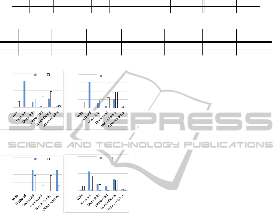
Table 6: Number of distinct values of OCC and SAL.
Age
Gender Marital Status Race Birth Place Education Work Class Occupation Income
80 2 6 9 124 24 9 50 50
Table 7: Number of distinct values of Adult data set.
Age
Work Class Final Weight Education Education-num Marital Status Occupation Relationship
74 7 26741 16 16 7 14 6
Race Gender Capital Gain Capital Loss Hours Per Week Country Salary Class
5 2 121 97 96 41 2
0
0.2
0.4
0.6
0.8
Ra o
Male Female
(a) Original database
0
0.2
0.4
0.6
0.8
Ra o
Male Female
(b) Estimated from the
anonymized database of
Proposal
0
0.2
0.4
0.6
0.8
Ra o
Male Female
(c) Estimated from the
anonymized database of TP
0
0.2
0.4
0.6
0.8
Ra o
Male Female
(d) Estimated from the
anonymized database of
Anatomy
Figure 6: Relationship vs. sex in l = 2.
onds. From this result, we know that our proposed
method is a very efficient technique in terms of exe-
cution time.
7 CONCLUSION
An anonymization technique of l-diversity can
achieve a privacy-preserving model where a data
holder can share their data with other data users. Ex-
isting techniques generalize QIDs from the database
to ensure that adversaries cannot specify each individ-
ual’s sensitive attribute. However, it is possible that
several QIDs that a data user focuses on are all gener-
alized and the anonymized database has no value for
the data user.
In this paper, we propose a new technique for l-
diversity, which keeps QIDs unchanged and random-
izes sensitive attributes of each individual so that data
users can analyze it based on QIDs that they focus on.
We also proposed an estimation protocol of the orig-
inal distribution of sensitive attributes for data users
according to their preferred QIDs, and, we proposed
the calculation method for the expected MSE between
the original and estimated distribution of sensitive
attributes. Moreover, our method does not require
the eligibility requirement, therefore, our method can
be applied to any databases when l is less than the
number of distinct sensitive values. By mathemati-
cal analysis and simulations, we prove that our pro-
posed method can result in a better tradeoff between
privacy and utility of anonymized databases than ex-
isting studies.
Future work will include the evaluation of other
relevant data sets. We also plan to extend our ap-
proach to other privacy measures such as t-closeness.
ACKNOWLEDGEMENTS
This research was subsidized by JSPS 24300005,
26330081, 26870201. The authors would also like
to express their deepest appreciation to the entire staff
of Professor Honiden’s laboratory at the University of
Tokyo and Professor Fukazawa’s lab at Waseda Uni-
versity, both of whom provided helpful comments and
suggestions.
REFERENCES
Cheong, C. H. (2012). Non-Centralized Distinct L-
Diversity. International Journal of Database Man-
agement Systems, 4(2):1–21.
Clifton, C. and Anandan, B. (2013). Challenges and Op-
portunities for Security with Differential Privacy. In
Information Systems Security, pages 1–13. Springer.
Domingo-Ferrer, J. (2013). On the Connection between t-
Closeness and Differential Privacy for Data Releases.
RandomizedAdditionofSensitiveAttributesforl-diversity
359

In Proc. International Conference on Security and
Cryptography (SECRYPT), pages 478–481.
Dwork, C. (2006). Differential Privacy. In Automata, Lan-
guages and Programming, volume 4052 of Lecture
Notes in Computer Science, pages 1–12. Springer.
Fung, B. and Yu, P. (2005). Top-Down Specialization for
Information and Privacy Preservation. In Proc. IEEE
ICDE, pages 205–216.
Fung, B. C. M., Wang, K., Chen, R., and Yu, P. S.
(2010). Privacy-preserving data publishing: A sur-
vey of recent developments. ACM Computing Sur-
veys, 42(4):1–53.
Ghinita, G. (2007). Fast Data Anonymization with Low
Information Loss. In Proc. VLDB, pages 758–769.
Groat, M. M., Edwards, B., Horey, J., He, W., and Forrest,
S. (2012). Enhancing privacy in participatory sens-
ing applications with multidimensional data. In Proc.
IEEE PerCom, pages 144–152.
Hu, H., Xu, J., On, S. T., Du, J., and Ng, J. K.-Y. (2010).
Privacy-aware location data publishing. ACM Trans.
Database Systems, 35(3):1–42.
Huang, Z. and Du, W. (2008). OptRR: Optimizing Random-
ized Response Schemes for Privacy-Preserving Data
Mining. In Proc. IEEE ICDE, pages 705–714.
Kabir, M., Wang, H., Bertino, E., and Chi, Y. (2010). Sys-
tematic clustering method for l-diversity model. In
ADC, volume 103, pages 93–102.
Kenig, B. and Tassa, T. (2011). A practical approximation
algorithm for optimal k-anonymity. Data Mining and
Knowledge Discovery, 25(1):134–168.
LeFevre, K., DeWitt, D., and Ramakrishnan, R. (2006).
Mondrian Multidimensional K-Anonymity. In Proc.
IEEE ICDE, pages 25–25.
LeFevre, K., DeWitt, D. J., and Ramakrishnan, R. (2008).
Workload-aware anonymization techniques for large-
scale datasets. ACM Trans. Database Systems,
33(3):1–47.
Li, N., Li, T., and Venkatasubramanian, S. (2007).
t-closeness: Privacy beyond k-anonymity and l-
diversity. In Proc. IEEE ICDE, pages 106–115.
Machanavajjhala, A., Kifer, D., Gehrke, J., and Venkita-
subramaniam, M. (2007). l-diversity: Privacy beyond
k-anonymity. ACM TKDD, 1(1):3–es.
Meyerson, A. and Williams, R. (2004). On the complexity
of optimal K-anonymity. In Proc. ACM PODS, pages
223–228.
Minnesota Population Center. Ipums,
https://www.ipums.org/.
Nergiz, A. E., Clifton, C., and Malluhi, Q. M. (2013). Up-
dating outsourced anatomized private databases. In
Proc. EDBT, page 179. ACM.
Nikolov, A., Talwar, K., and Zhang, L. (2013). The geome-
try of differential privacy: the sparse and approximate
cases. In Proc. ACM STOC, pages 351–360.
Samarati, P. (2001). Protecting respondents identities in mi-
crodata release. IEEE Trans. Knowledge and Data En-
gineering, 13(6):1010–1027.
Sun, X., Wang, H., Li, J., and Ross, D. (2009). Achieving P-
Sensitive K-Anonymity via Anatomy. In Proc. IEEE
International Conference on e-Business Engineering
(ICEBE), pages 199–205.
Sweeney, L. (2002). Achieving k-anonymity privacy pro-
tection using generalization and suppression. In-
ternational Journal of Uncertainty, Fuzziness and
Knowledge-Based Systems, 10(05):571–588.
UCI Machine Learning Repository. Adult Data Set,
http://archive.ics.uci.edu/ml/datasets/Adult.
Wu, S., Wang, X., Wang, S., Zhang, Z., and Tung,
A. K. (2013). K-Anonymity for Crowdsourcing
Database. IEEE Trans. Knowledge and Data Engi-
neering, PP(99).
Xiao, X. and Tao, Y. (2006). Anatomy: simple and effective
privacy preservation. In Proc. VLDB, pages 139–150.
Xiao, X., Yi, K., and Tao, Y. (2010). The hardness and
approximation algorithms for l-diversity. In Proc.
EDBT, pages 135–146.
Xie, H., Kulik, L., and Tanin, E. (2011). Privacy-aware col-
lection of aggregate spatial data. Data & Knowledge
Engineering, 70(6):576–595.
Yao, L., Wu, G., Wang, J., Xia, F., Lin, C., and Wang, G.
(2012). A Clustering K-Anonymity Scheme for Loca-
tion Privacy Preservation. IEICE Trans. Information
and Systems, E95-D(1):134–142.
SECRYPT2014-InternationalConferenceonSecurityandCryptography
360
