
Evolutionary Algorithms Applied to Agribusiness Scheduling Problem
Andre Noel, Jos
´
e Magon Jr. and Ademir Aparecido Constantino
Computer Science Department, Maringa State University, Av. Colombo, 5790, Maringa, PR, Brazil
Keywords:
Operational Research, Scheduling, Evolutionary Algorithms, Genetic Algorithms.
Abstract:
This paper addresses a scheduling problem in agribusiness context, especifically about chicken catching. To
solve that problem, memetic algorithms combined with local search in a two-phase algorithm were proposed
and investigated. Four versions of memetic algorithms were implemented and compared. Also, to apply
local search, k-swap and SRP is proposed and experimented. At last we analyze the results, comparing perfor-
mances. The obtained results show a good improvement in solutions, especially when compared to the manual
scheduling actually performed by the company that provides the data to this study.
1 INTRODUCTION
Scheduling Problem (SP) is a common name to a
computing problem set, often at NP-hard class, which
has the purpose of allocate event or resource sets
throughout a time period, satisfying a set of con-
straints, usually to optimize a fitness function. That
resource might be persons, machines, vehicles, phys-
ical location, etc. The SP class arises from real prob-
lems on industry and organizations. These problems
are also observed on software engineering, according
(Xiao et al., 2013). The main challenge is usually
to find a computational methodology to solve these
problems in a efficient and effective way, making pos-
sible to generate computational systems to automate
real-problem resolutions.
In this paper, we examine a SP class variant, the
Agribusiness Scheduling Problem (ASP), at a Poultry
Industry context. It is a combinatorial optimization
problem with great computational complexity which
has been poorly addressed (Hart et al., 1999; Con-
stantino et al., 2011). The ASP is shown as a NP-
complete problem, as the mostly of scheduling prob-
lems (Bodin, 1983), without any polynomial-time
complexity algorithm that solves it with an optimal
solution.
The purpose of this work is to compare some evo-
lutionary algorithms applied to the ASP. So, in Sec-
tion 2 is explained what do we expect from a shift at
the chicken factory. In Section 3 the problem is de-
scribed in a way we can develop a solution, which is
proposed in Section 4. In Section 5 we discuss the ex-
periments and the obtained results. At the end, some
conclusions in Section 6.
2 CHICKEN CATCHING SQUAD
SCHEDULING
Our problem occurs on agribusiness context, dealing
with chicken transport to the factories. As chickens
are fragile animals, they can’t stay longer at the lor-
ries, exposed to high temperatures. So, the squad’s
shift for transport and discharging must be careful
planned to not create long queues at the factories.
There are different farms, which has different dis-
tances to the factories. When they get at the right age,
they will be catched and sent to slaughter.
Also, we have the catcher squads, who are respon-
sible to catch the chickens to transport them to the
factories. To generate the schedule, we need to ob-
serve labor law and constraints about work time and
rest time.
At last, the vehicles to transport the chickens must
be considered, calculating the capacity, velocity and
availability. All that factors may change the problem
modeling.
3 PROBLEM DESCRIPTION
The problem described here is a real-world schedul-
ing problem of a brazilian company, which daily has
to catch chicken at different farms and carry them to
three factories (slaughterhouses).
489
Noel A., Magon Jr. J. and Constantino A..
Evolutionary Algorithms Applied to Agribusiness Scheduling Problem.
DOI: 10.5220/0004895104890496
In Proceedings of the 16th International Conference on Enterprise Information Systems (ICEIS-2014), pages 489-496
ISBN: 978-989-758-027-7
Copyright
c
2014 SCITEPRESS (Science and Technology Publications, Lda.)

The farms are located far from until 150 km of
each factory and different farms can be added to the
problem. So, the schedule has to be daily generated
according all different variables.
There are some squads to travel from their base to
the farms. A squad must travel to one farm, catch the
chickens, load the lorries and travel to the next farm
to do the same.
The lorries and drivers will be considered as an
unique entity, so we’ll just think about the lorry,
which may have known capacity and average velocity.
Also, the distance between each farm to the factories
is known.
Our work has to determine what load will be de-
signed to each factory and the schedule to minimize
the costs of idle factories and paid time. So, the
catches and the travels has to be calculated in a way
to avoid long queues at the factories and to catch the
chickens at the right moment.
The factories has a ventilated hangar where the
lorries can wait a determined period. Obviously it has
a limited size, so our goal is to not admit more lorries
at the queue than the hangar capacity. And even be-
ing ventilated there is a time limit that the the chickens
can wait.
Figure 1 illustrates how it all works. At this exam-
ple, we have two squads to catch the chickens to three
factories. The continuous lines represent the travel
sequence of each squad and the dashed lines repre-
sent the lorries’ travels carrying the chickens from the
farms to the factories. Also, the squads’ bases are in
different locations from the factories. Thus, we’re in-
terested on find some informations as the sequence of
the farms to each squad, the squads’ initial and final
work times, the time of lorries’ load and the destina-
tion of each load.
Figure 1: Daily the squads go to the farms, to catch the
chickens and load the lorries, which carry them to the facto-
ries. When they finish the load, the squad travel to the next
farm at the schedule.
To get clear, our purpose is to minimize the costs,
minimizing the work time and the idle time. To
achieve this, we have to observe some restrictions and
local laws, but we won’t take time explaining they at
this work.
4 PROPOSAL
In our approach the problem is divided into several
subproblems. At this section we present the first
subproblem solved, that is the assignment problem,
which assign each farm load to one factory. After, we
present the subproblems of the initial solutions and
the local search. At last, the general algorithm to gen-
erate solutions to the general problem.
4.1 The Assignment Problem
To solve the load’s destination subproblem, we use
a mathematical model. This model is similar to the
Zero-One Knapsack Problem (Kellerer et al., 2004).
We get the loads by dividing the number of chick-
ens by the lorry capacity. Here we suppose an equal
capacity for the lorries. Each load is associated to:
• Origin (farm);
• Destination (factory);
• Load start time;
• Load duration;
• Responsible squad; and
• Number of chickens.
As we know the farm set and their informations, as
location and number of chickens, the number of loads
and load duration are automatically retrieved. So, we
still need to discover the destination, the squad and
the start time to catch the chickens.
Then, to minimize the costs, a fundamental phase
is to find the assignment of the loads to the factories.
To do this, we use a binary integer linear program-
ming model which is solved using LP-Solve software.
But this model solves just part of the problem, mini-
mizing transport costs only. Still, the scheduling has
to be solved by using heuristic algorithms.
The evolutive algorithms in this paper use the lin-
ear assignment model on two phases: at the con-
struction phase and at the improvement phase (local
search). The assignment problem (AP), denoted by
PD([C
i j
]), is the following:
Min
n
1
∑
i=1
n
2
∑
j=1
c
i j
x
i j
ICEIS2014-16thInternationalConferenceonEnterpriseInformationSystems
490

Sub jectto :
n
1
∑
i=1
x
i j
= 1, ∀ j = 1, . . . , n
2
n
2
∑
j=1
x
i j
= 1, ∀i = 1, . . . , n
1
x
i j
∈ 0, 1, ∀i = 1, . . . , n
1
, ∀ j = 1, . . . , n
2
Let be x
i j
is a binary decision variable {0, 1},
where x
i j
= 1 if i is associated to j, or x
i j
= 0 oth-
erwise. And let be c
i j
the cost to associate i to j.
The n
1
value must be the same as n
2
value. At the
first phase, n
1
represents the number of squads and
n
2
the number of loads. As the number of loads is
always greater than the number of squads, thus ficti-
tious squads are created to get a squared matrix [c
i j
].
At improvement phase, n
1
and n
2
are always the max-
imum number of squads (ne
max
) allowed for schedul-
ing. Even though the algorithm takes the max number
of available squads, the goal is to minimize the global
cost of human resources. This model is used both on
construction and improvement phases.
In order to generate the scheduling, we can de-
fine it as an activity sequence to be taken throughout
the day, with average lorry loading time of about one
hour. So, to simplify our problem, we can discretize
the day on one-hour time slot. Thus, we consider t as
the time index, with t = 1,...,24, where t = 1 represents
the first time slot of the day, when some squad starts
its work.
4.2 Construction Phase
We can use the assignment model to create the initial
solution. Initially, all sequence of each squad (from
ne
max
squads) are empty. So, the loads are succes-
sively assigned to the squads until assign to all squads,
using t = 1, starting the squad work at the first time
slot. As we always have more loads than squads, to
the others time slots (t > 1) the assignment is solved
using the assignment problem.
After the initial process, we get a initial schedule,
as illustrated by Figure 2.
Figure 2: Example of an initial load distribution among the
squads.
4.3 Local Search
From initial solution, local search is a good method
to get improved solutions. In this work we use search
procedures based on VND (Variable Neighborhood
Descent), a particular case of Variable Neighborhood
Search (Hansen and Mladenovi
´
c, 2001).
4.3.1 k-swap
The first local search method we used is the k-swap,
which consists on slice our schedule on k time slots,
starting at a t time, generating activity blocks. So, k-
swap investigates the swaps between the blocks to get
a improved solution.
The investigation uses successive assignment
problems, calculating the cost of assignment to dif-
ferent instances. Considering st as the starting time at
the squads schedules and et the end time, or the last
time slot of work, we can write the k-swap algorithm
as follows.
start;
z∗ ← ∞;
for t ← (st + 1) to (et - k - 1) do
Creates a cost matrix [c i j] to load ba(k, t);
Solves assignment problem AP([c i, j]);
if z < z∗ then
z∗ ← z; //saving the best z value till now
t∗ ← t; //saving the best t value till now
end if
end for
Associates loads to squads according AP([c i, j])
on t∗;
end
Figure 3 illustrates an example of 1-swap for t
= 4, using a graph to represent the activities that 4
squads would perform in a seven-hour period to load
18 loads. The labeled vertices represent the loads,
while blank vertices represent time slots without any
loading (rest or travel). The continuous edges rep-
resent the predefined activity sequence and dashed
edges represents the possible swaps.
Figure 3: 1-swap considering only one interval at t = 4.
At Figure 4, we observe an example of 2-swap,
considering times t = 4 and t = 5, using consecutive
time slots.
EvolutionaryAlgorithmsAppliedtoAgribusinessSchedulingProblem
491

Figure 4: 2-swap considering the consecutive intervals t = 4
and t = 5.
4.3.2 Split and Recombination Procedure
Another local search investigated is the Split and Re-
combination Procedure (SRP). This procedure works
slicing the schedule between two work times, dividing
the schedule on two parts, and recombines it using the
assignment problem. Figure 5 illustrates that process.
Figure 5: SRP applied at interval between t = 1 and t = 2.
4.3.3 bl-VND General Algorithm
The bl-VND algorithm is based on VND (Variable
Neighborhood Descent), which explores the solution
space with systematic neighborhood changes (Hansen
and Mladenovi
´
c, 2001), if current solution weren’t
improved on a particular neighborhood, a next neigh-
borhood is explored and so on. Let’s state R as the
neighborhood set, N
1
, N
2
, . . . , N
R
. On our algorithm,
we use R = 6, where N
1
= 1-swap, N
2
= 2-swap, . . . ,
N
5
= 5-swap and N
6
= SRP.
Each iteration of bl-VND explores all neighbor-
hoods and the algorithm stops when no improvement
occurs on any of iterations. The algorithm is pre-
sented below.
start
Initialization:
start
selects a neighborhood structure set N,
(r = 1, ..., 6);
selects a initial solution S;
end
repeat
r ← 1;
repeat
Local search: Find s’ solution from s
(s’ ∈ N r(s));
if f1(s’) < f1(s) then
s ← s
0
;
r ← 1;
end if
else
r ← r + 1;
end else
until r = R;
until satisfies break criteria;
end
4.4 Local Search at Queues
The construction phase and the previous local
searches aim to minimize the costs with paid time.
So, until now we didn’t consider the impact on the
factories’ work, as idle time or lorries’ wait time at
the queues.
To take care of that problem a penalty was intro-
duced to evaluate the idle time under our objective
function.
Then, to minimize the idle time and the wait time
at the hangars, a local search algorithm, named bl-
Queue, was designed. The main role of it is to change
the initial time of each squad’s schedule, in order to
don’t have many loads waiting at the same time on the
same factories.
bl-Queue algorithm then evaluates the impact of
each schedule starting at the times t = 1, . . . ,t
max
,
where t
max
is the max time allowed to unload the loads
on time to slaughter. This is done successively to each
of the squads. The below algorithm presents how bl-
Queue works.
start;
for s ← 1 to sn do
Finds a t time to starts the schedule
to s squad with minor cost;
Changes s initial time to t;
end for
end
To determine the time of the queues, a simulation
is performed, using the 3-phases method (Medina and
Chwif, 2007). In short, this method does:
• Checks the time of all events in schedule to select
the one who occurs first. Update the simulation
clock to the selected time.
• Executes the selected event and the entities (loads)
are moved to the waiting queues to the next activ-
ity.
• Searchs the entities at the queue and starts the
events that satisfies current conditions. Moves the
entities from queues to activities and calculates
the time each entity stayed at the queues.
The loads analyzed before can be the entities
whose realizes the simulation events. Once we know
the squads initial work time, is possible to deter-
mine at what time the loads will arrive at the desti-
nation. So, we can calculate how many time each en-
tity stayed at queue. At the end of simulation we get
ICEIS2014-16thInternationalConferenceonEnterpriseInformationSystems
492
statistics about the queues, as total time of wait and
average queue size.
4.5 Memetic Algorithms
Memetic Algorithms belongs to the populational al-
gorithms class. It uses several solutions searching
feasible solutions in a search space. The main fea-
ture of that approach is to uses hybridization of differ-
ent algorithmic techniques to a specific problem (Neri
et al., 2011).
That class of algorithms was introduced by
Moscato (Moscato, 1989) describing an evolutionary
process that uses local search as a decisive part of the
evolution. It may be seen as an local refinement inside
a search space, in a way an agent can has his adaption
level increased after a refinement stage.
The fundamentals of Memetic Algorithms con-
sists on combine different meta-heuristics concepts
and strategies, as the population-based search with lo-
cal search, intending to join the advantages of them
(Neri et al., 2011).
Four different versions of Memetic Algorithms
were developed in this work. They’re evolutive al-
gorithms with construction procedures, local search
and other techniques. The new algorithms are: Hi-
erarchical Memetic Algorithm (HMA), Hierarchical-
generational Memetic Algorithm (HGMA), Alternate
Memetic Algorithm (AMA) and Coevolutive Cooper-
ative Memetic Algorithm (CCMA).
5 EXPERIMENTS AND RESULTS
Some experiments were performed in order of an-
alyze and compare different implementations. The
four memetic algorithms of previous section were
used, as the existing version proposed by (Con-
stantino et al., 2011).
First of all, we define the parameters. Then we
analyze the impact of local search. At last, we show
the results using real data.
5.1 Defining Parameters
To perform the experiments, we had to set up all the
parameters in a way to get a better performance using
genetic algorithms.
As observed, the crossing genetic operator gener-
ates many infeasible solutions. So, empirically, was
defined a Crossover Rate of 100% to force the algo-
rithm to always use that operator.
After some experiments to calibrate our parame-
ters and some statistical analysis, we adjust the algo-
rithm parameters as showed on Table 1.
Table 1: Initial parameters for genetic algorithm.
Parameter Value
Population size 120
Mutation tax 3%
Number of iterations (MaxIt) 2000
Ω 50%
5.2 Local Search Impact
To identify the real contribution of local search to ob-
tain the solutions, a experiment was performed with
the aim to quantify the acting of the search at each
current best global solution, comparing to the other
solutions obtained by genetic algorithm.
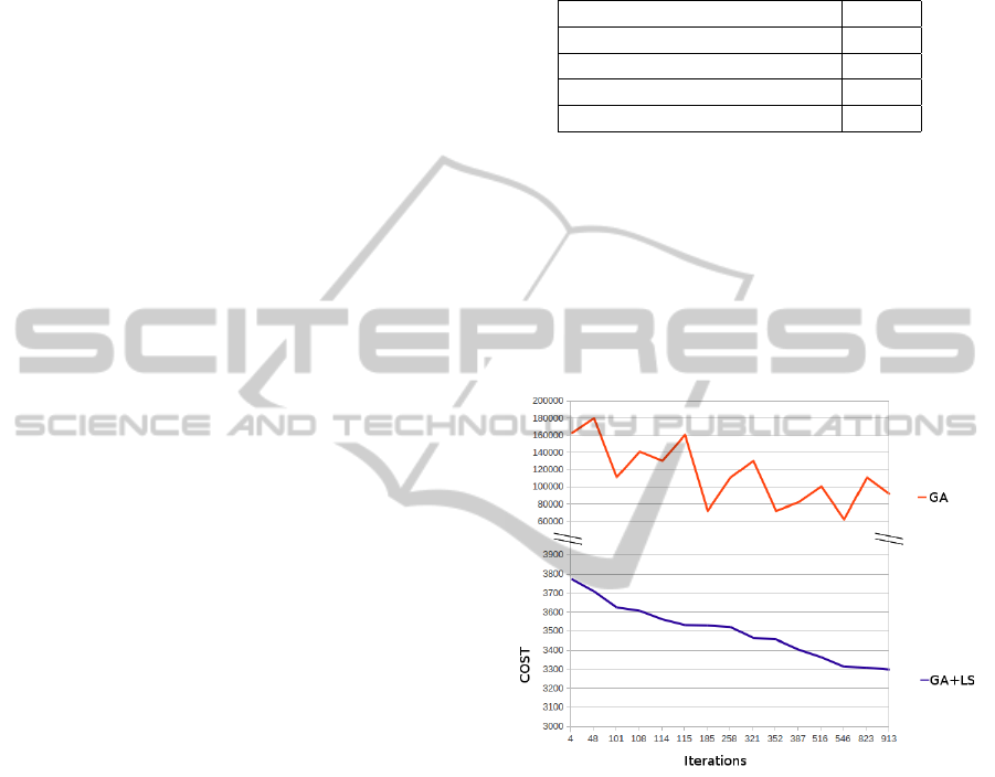
The Figures 6, 7 and 8 show graphs generated
from tests using real data for test cases A, B and C.
Figure 6: Obtained results using GA and GA + Local
Search - Test case A.
Two scales were used for cost axis, because there
is a great distance between costs of using only GA or
GA combined with local search. After analyze these
graphs, we observed that the genetic algorithms have
the task to create potential good solutions, not nec-
essarily having good costs, whilst local search algo-
rithms are responsible to get solutions with acceptable
costs.
Another observation at these graphs is that in none
of the cases the solution was improved after 1000 it-
erations. Even though, there are some cases where
higher values of iterations has proved to be useful.
5.3 Computional Results
The experiments were performed using a CPU Intel
EvolutionaryAlgorithmsAppliedtoAgribusinessSchedulingProblem
493

Figure 7: Obtained results using GA and GA + Local
Search - Test case B.
Figure 8: Obtained results using GA and GA + Local
Search - Test case C.
Core I5, 2.3 GHz, under Ubuntu 11.04 64 bits, ker-
nel Linux 2.6.38, using C++ language, compiled with
GCC, from GNU. These experiments used real data,
collected from a real company over a three months
operation period (62 data instances). This period in-
volves 112 catchers, divided on squads of 14 persons
(including the driver).
To solve the mathematical model we used the LP-
Solve, a solver used to solve linear models, non-linear
models and integer mathematical programming, as
the proposed model.
A implementation of Kuhn-Munkres algorithm
(Kuhn, 1955), also known as Hungarian Algorithm,
was used to solve the Assignment Problem.
At Table 2 shows the instances used to the experi-
ments. Each instance represents a work day. So, at the
table is possible to observe the problem size, observ-
ing how many farms (fq) and loads (oq) are involved.
Table 2: Instances of the problem used on the experiments.
Instance fq oq Instance fq oq
1 10 48 32 7 52
2 9 46 33 6 52
3 9 47 34 5 44
4 8 44 35 5 38
5 9 50 36 7 54
6 9 48 37 7 26
7 10 46 38 5 42
8 6 37 39 9 48
9 7 52 40 8 55
10 6 43 41 9 53
11 7 47 42 8 45
12 5 37 43 10 57
13 6 46 44 12 55
14 5 37 45 9 43
15 5 49 46 8 35
16 5 38 47 9 42
17 4 49 48 12 41
18 7 49 49 8 45
19 7 43 50 10 45
20 10 44 51 7 52
21 5 44 52 9 47
22 2 45 53 5 49
23 4 46 54 7 46
24 4 39 55 6 50
25 7 41 56 7 54
26 7 53 57 6 49
27 5 52 58 7 44
28 4 52 59 7 46
29 3 37 60 3 26
30 4 46 61 2 16
31 7 54 62 8 54
Overall, the average of farms visited by day is 6.8,
with an average of 45.4 loads transported.
5.4 Explained Results
Table 3 shows the obtained results separated by
the different implementations of memetic algorithms.
Explaining, we have:
• The results about total distance traveled are the
same in all versions because it’s obtained from the
same mathematical model.
• Although the computational time has vary among
the versions, in no one the time has increased in a
way that prejudices any version. It all finished in
a feasible computational time.
• The Manual column has the cost of the original
scheduling, manually generated by the company.
• The HMA column shows the results using the
HMA algorithm with initial parameters configu-
ration.
• The AHMA column shows the results using the
ICEIS2014-16thInternationalConferenceonEnterpriseInformationSystems
494

Table 3: Results summary from performed implementations.
Manual HMA AHMA HGMA AMA CCMA
Total paid
4060.25 3843.45 3766.54 3672.29 3837.28 3656.51
time (hours)
Total dist.
370436.8 347834.4 347834.4 347834.4 347834.4 347834.4
travelled (km)
Total idle
60.12 17.15 14.68 6.03 17.21 0.00
time (hours)
Avg lorries
4.01 2.35 2.14 2.48 3.74 2.24
at queue
Avg wait
119.04 4.33 4.33 26.82 26.24 4.93
time (minutes)
Lorries overflow
92 9 8 2 10 0
at queue
Infeasible schedule
51 7 7 4 13 0
quantity
Computational
- 115 130 160 120 180
time (minutes)
Table 4: Qualitative results for some instances of the problem.
Manual HMA AHMA HGMA AMA CCMA
Instance A
Factory got stopped? Y Y N N Y N
Got lorries overflow? Y Y Y N Y N
Was schedule infeasible? Y Y Y Y Y N
Instance B
Factory got stopped? Y Y Y Y Y N
Got lorries overflow? Y Y N N Y N
Was schedule infeasible? Y Y Y Y Y N
Instance C
Factory got stopped? Y Y Y N Y N
Got lorries overflow? Y Y Y Y Y N
Was schedule infeasible? Y Y Y N Y N
Adjusted-HMA algorithm, which has the parame-
ters adjusted, as shown at section 5.1 (Table 1)
• From HGMA column, we observe that the Gen-
erational approach provides better results, despite
of a increasing at the wait time at the factories.
• The AMA column shows the results using the
AMA algorithm, based on joining both phases of
HMA algorithm, but it didn’t improves the results,
getting worse at some aspects.
• The CCMA column shows the results using the
CCMA algorithm, based on coevolutive and pre-
vious versions to get a version that presented the
best results. It shows evidences that this approach
is more flexible and makes a better exploration of
the search space.
5.5 About CCMA Version
The main contribution of CCMA version is the better
performance to generate scheduling to the test cases
previous versions was not able to find good solutions.
Table 4 shows qualitative results about proposed
algorithms to some instances of the problem.
Table 5 compares CCMA results with the manual
scheduling generated by the company, evaluating the
difference between the solutions.
The results present a significant reduction of oper-
ational costs. The paid time is related to the squads,
so the cost must be multiplied by 14, the number of
persons at each squad.
Also, it reduces infeasible duties, which are sched-
ules with erroneous calculation of travel time between
farms. It generates extra costs to the company. 100%
of these cases were reduced using CCMA. Still it re-
moves some undesirable schedules, with long work
time without rest.
The factories idle time was also reduced to zero.
The cost of an idle factory is usually very high, reach-
ing the value of US$6000.00/hour.
It still reduces the number of lorries parked in the
factories’ hangars in about 50% and the average wait
time was reduced in more than 95%. Also, a reduction
of 100% of the lorries overflow. When more lorries
EvolutionaryAlgorithmsAppliedtoAgribusinessSchedulingProblem
495

Table 5: Comparison between manual and CCMA computational scheduling.
Manual CCMA Reduction % reduction
Total paid
4060.25 3656.51 403.74 9.94
time (hours)
Total dist.
370436.8 347834.4 22602.4 6.1
travelled (km)
Total idle
60.12 0.00 60.12 100
time (hours)
Avg lorries
4.01 2.24 1.77 44.1
at queue
Avg wait
119.04 4.93 114.11 95.86
time (minutes)
Lorries overflow
92 0 92 100
at queue
Infeasible schedule
51 0 51 100
quantity
are stopped than the factory capacity, the lorry has to
go to some unappropriated place, which may cause
chickens mortality and increase of operational costs.
6 CONCLUSIONS
This work presented a study on heuristic algorithms
to solve a scheduling problem in agribusiness context.
After all study and experiments, we can conclude:
• Memetic algorithms had an important role in this
work due their flexibility and facility to incor-
porate new procedures. Also, they ease solving
problems with hard mathematical modeling.
• Performed experiments had demonstrated the fea-
sibility of using computational systems to auto-
mate the schedule generation to solve real prob-
lems.
• Local search had a great importance to reduce the
costs on obtained solutions.
• Comparing the obtained solutions with manual
solutions of the company, evolutive algorithms
had a very great reduction on operational costs,
generating schedules in feasible computational
time. The final solutions presents improvements
both on quality and in reduction of the costs.
REFERENCES
Bodin, L. (1983). Solving large vehicle routing and
scheduling problems in small core. In Proceedings of
the 1983 annual conference on Computers: Extending
the human resource, pages 27–37. ACM.
Constantino, A. A., Landa-Silva, D., and Rom
˜
ao, W.
(2011). Algoritmo evolutivo h
´
ıbrido para escalon-
amento integrado na agroind
´
ustria. In Computac¸
˜
ao
Evolucion
´
aria em Problemas de Engenharia, pages
251–272. Omnipax.
Hansen, P. and Mladenovi
´
c, N. (2001). Variable neighbor-
hood search: Principles and applications. European
journal of operational research, 130(3):449–467.
Hart, E., Ross, P., and Nelson, J. A. (1999). Scheduling
chicken catching-an investigationinto the success of a
genetic algorithm on areal-world scheduling problem.
Annals of Operations Research, 92:363–380.
Kellerer, H., Pferschy, U., and Pisinger, D. (2004). Knap-
sack Problems. Springer.
Kuhn, H. W. (1955). The hungarian method for the as-
signment problem. Naval research logistics quarterly,
2(1-2):83–97.
Medina, A. and Chwif, L. (2007). Modelagem e simulac¸
˜
ao
de eventos discretos: teoria & aplicac¸
˜
oes.
Moscato, P. (1989). On evolution, search, optimization, ge-
netic algorithms and martial arts: Towards memetic
algorithms. Caltech concurrent computation program,
C3P Report, 826:1989.
Neri, F., Cotta, C., and Moscato, P. (2011). Handbook of
memetic algorithms, volume 379. Springer.
Xiao, J., Ao, X.-T., and Tang, Y. (2013). Solving soft-
ware project scheduling problems with ant colony op-
timization. Comput. Oper. Res., 40(1):33–46.
ICEIS2014-16thInternationalConferenceonEnterpriseInformationSystems
496
