TrieMotif

A New and Efﬁcient Method to Mine Frequent K-Motifs from Large Time Series

Daniel Y. T. Chino

, Renata R. V. Gonc¸alves

, Luciana A. S. Romani

Caetano Traina Jr.

and Agma J. M. Traina

Institute of Mathematics and Computer Science, University of S

ao Paulo, S

ao Carlos, Brazil

Cepagri-Unicamp, Campinas, Brazil

Embrapa Agriculture Informatics, Campinas, Brazil

Keywords:

Time Series, Frequent K-Motif, AVHRR-NOAA Images.

Abstract:

Finding previously unknown patterns that frequently occur on time series is a core task of mining time series.

These patterns are known as time series motifs and are essential to associate events and meaningful occurrences

within the time series. In this work we propose a method based on a trie data structure, that allows a fast and

accurate time series motif discovery. From the experiments performed on synthetic and real data we can see

that our TrieMotif approach is able to efﬁciently ﬁnd motifs even when the size of the time series goes longer,

being in average 3 times faster and requiring 10 times less memory than the state of the art approach. As a

case study on real data, we also evaluated our method using time series extracted from remote sensing images

regarding sugarcane crops. Our proposed method was able to ﬁnd relevant patterns, as sugarcane cycles and

other land covers inside the same area.

1 INTRODUCTION

The large volume of time series continually generated

by a variety of sensors, climate models and stock mar-

kets demands fast methods to take advantage of such

amount of data. The information contained in time

series databases is a rich source for decision making

tasks demanded by the owners of such data. One of

the main tasks when mining time series is to ﬁnd the

motifs present therein, that is, to ﬁnd patterns that fre-

quently occurs in time series. By ﬁnding motifs, it

is possible to mine association rules aimed at spotting

patterns indicating that some events frequently lead to

others.

Existing applications involving time series, such

as stock market analysis, are not yet able to record all

the factors that govern the data organized in the time

series, such as political and technological factors. On

the contrary, climate variations nowadays have most

of its governing factors being recorded, using sens-

ing equipments such as satellites and ground-based

weather stations. However, the diversity of data avail-

able makes it hard to discover complex patterns that

can support more robust analyzes. In this scenario,

ﬁnding motifs assumes an even greater importance.

In this work we took advantage of real time se-

ries extracted from remote sensing imagery contain-

ing Normalized Difference Vegetation Index (NDVI)

measurements. The NDVI time series present the veg-

etative strength of the plantation (Rouse et al., 1973).

To follow the development of a crop is strategic for

agribusiness practices in Brazil, since agriculture is

the country’s main asset. The accurate monitoring of

agriculture in the whole world have become more and

more important specially due to climate change im-

pacts. The “food safety” issue has concerned gov-

ernments from several countries and the development

of new technologies for monitoring, as well as the

proposition of mitigation and adaptation measures,

are crucial. In this sense, remote sensing can be an im-

portant tool to improve the fast detection of changes

in the land cover besides to aid at monitoring the crop

cycle.

Since the volume of time series databases as well

as the length of the series is growing at a very fast

pace, it is mandatory to develop algorithms and meth-

ods that can deal with time series in the scenario of

big data. In this paper we present a new method to

extract motifs from time series and a new algorithm

to index them in a trie data structure that performs

well over large time series, which is up to 3 times

faster than the state-of-the-art method. We evaluated

Chino D., Gonçalves R., Romani L., Traina Jr. C. and Traina A..

TrieMotif - A New and Efﬁcient Method to Mine Frequent K-Motifs from Large Time Series.

DOI: 10.5220/0004891900600069

In Proceedings of the 16th International Conference on Enterprise Information Systems (ICEIS-2014), pages 60-69

ISBN: 978-989-758-027-7

 2014 SCITEPRESS (Science and Technology Publications, Lda.)

the proposed TrieMotif over both synthetic and real

time series and obtained very promising results.

This paper is organized as follows. Section 2 sum-

marizes the main concepts used as the basis to de-

velop our work. Section 3 describes our proposed

method and Section 4 discusses its evaluation. Sec-

tion 5 shows the TrieMotif performance on real data

obtained from remote sensing images and Section 6

concludes this paper.

2 BACKGROUND AND RELATED

WORKS

A time series motif is a pattern that occur frequently.

They were ﬁrst deﬁned in (Lin et al., 2002) and a gen-

eralized deﬁnition was given in (Chiu et al., 2003). In

this section we recall these deﬁnitions and notations,

as they will be used in this paper. First we begin with

a deﬁnition of time series:

Deﬁnition 1. Time Series: A time series T =

, . . . ,t

is an ordered set of m real-valued variables.

Since we want to ﬁnd patterns that frequently oc-

cur along a time series, we will not work with the

whole time series, we are aiming only at parts of a

time series, which are called subsequences and are de-

ﬁned as follows.

Deﬁnition 2. Subsequence: Given a time series T

of length m, a subsequence S

of T is a sampling

of length n < m of contiguous positions from T be-

ginning at position p, that is, S

= t

, . . . ,t

p+n−1

for

1 ≤ p ≤ m − n + 1.

In order to ﬁnd frequent patterns, we need to de-

ﬁne a matching between patterns.

Deﬁnition 3. Match: Given a distance function

D(S

, S

) between two subsequences, a positive real

number R (range) and a time series T containing a

subsequence S

and a subsequence S

, if D(S

, S

) ≤

R then S

is called a matching subsequence of S

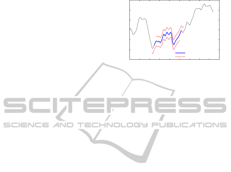
On subsequences of the same time series, the best

matches are probably subsequences that are slightly

shifted. Matching between two overlapped subse-

quences is called a trivial match. Figure 1 illustrates

the idea of a trivial match. The trivial match is deﬁned

as follows:

Deﬁnition 4. Trivial Match: Given a time series T ,

containing a subsequence S

and a matching subse-

quence S

, we say that S

is a trivial match to S

if ei-

ther p = q or if there is no subsequence S

beginning

at q

such that D(S

, S

) > R, and either q < q

< p

or p < q

< q. That is, if two subsequences overlaps,

-30

-20

-10

0 20 40 60 80 100 120 140 160 180

Time

Trivial Match

Figure 1: The best matches of a subsequence S

are proba-

bly the trivial matches that occur right before or after S

there must exist a subsequence between them that is

not a match.

These deﬁnitions allow deﬁning the Frequent K-

Motif problem. First, all subsequences are extracted

using a sliding window. Then, since we are inter-

ested in patterns, each subsequence is z-normalized

to have zero mean and one standard deviation (Keogh

and Kasetty, 2003). The K-Motif is deﬁned as fol-

lows.

Deﬁnition 5. Frequent K-Motifs: Given a time series

T , a subsequence of length n and a range R, the most

signiﬁcant motif in T (1-Motif ) is the subsequence

{1}

that has the highest count of non-trivial matches.

The K

most signiﬁcant motif in T (K-Motif ) is the

subsequence F

{K}

that has the highest count of non-

trivial matches, and satisﬁes D(F

{K}

, F

{i}

) > 2R, for

all 1 ≤ i < K.

The Nearest Neighbor motif was deﬁned by

Yankov et al. (Yankov et al., 2007), and it represents

the closest pair of subsequences. In our proposed

work, we focus on the Frequent K-Motif problem and

we will be referring to them as K-Motif. Since the K-

Motifs are unknown patterns, a brute-force approach

would compare every subsequence with each other.

This approach has quadratic computational cost since

it requires O(m

) calls to the distance function.

An approach to reduce the complexity of this

problem employs dimensionality reduction and dis-

cretization of the time series (Lin et al., 2002).

The SAX (Symbolic Aggregate approXimation) tech-

nique allows time series of size n to be represented by

strings of arbitrary size w (w < l) (Lin et al., 2003).

For a given time series, SAX consists of the follow-

ing steps. Firstly, the time series is z-normalized, so

that the data follow normal distribution (Goldin et al.,

1995). Next, the normalized time series is converted

into the Piecewise Aggregate Approximation (PAA)

TrieMotif-ANewandEfﬁcientMethodtoMineFrequentK-MotifsfromLargeTimeSeries

representation, decreasing the time series dimension-

ality (Keogh et al., 2001). The time series is then re-

placed with w values corresponding to the average of

the respective segment. Thus, in the PAA representa-

tion, the time series is divided into w continuous seg-

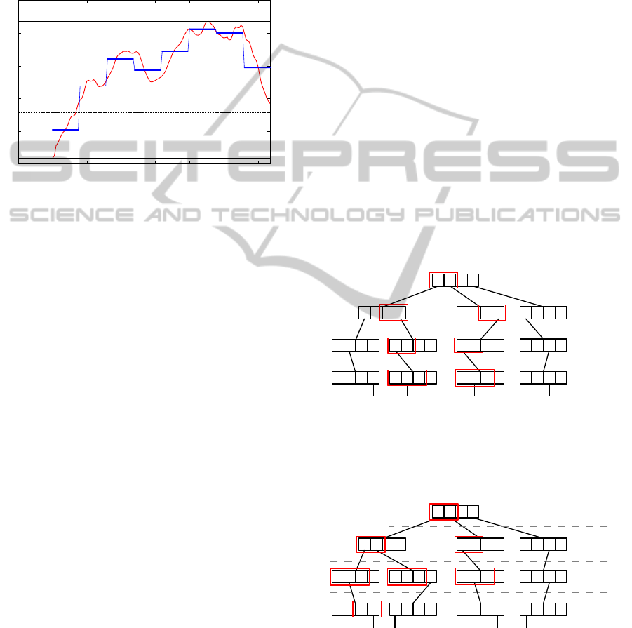
ments of equal length. Finally, the PAA representa-

tion is discretized into a string with an alphabet of size

a > 2. Figure 2 shows an example of a time series sub-

sequence of size n = 128 discretized using SAX with

w = 8 and a = 3. It is also possible to compare two

SAX time series using the MINDIST function. The

MINDIST lower bounds the Euclidean distance (Lin

et al., 2007), warranting no false dismissals (Falout-

sos et al., 1994).

-3

-2

-1

0 20 40 60 80 100 120

Time

Figure 2: A time series subsequence of size n = 128 is re-

duced to a PAA representation of size w = 8 and then is

mapped to a string of a = 3 symbols AABBCCCB.

Chiu et al. proposed a fast algorithm based on

Random Projection (Chiu et al., 2003). Each sub-

sequence of a time series is discretized using SAX.

The discretized subsequences are mapped into a ma-

trix, where each row points back to the original po-

sition of the subsequence on the time series. Then,

the algorithm uses the random projection to com-

pute a collision matrix, which counts the frequency

of subsequence pairs. Through the collision matrix,

the subsequences are checked on the original domain

seeking for motifs. Although fast, the collision ma-

trix is quadratic on the length of the time series, re-

quiring a high amount of memory. Also using the

SAX discretization, Li and Lin (Li and Lin, 2010;

Li et al., 2012) proposed a variable length motif dis-

covery based on grammar induction. Catalano et al.

(Catalano et al., 2006) proposed a method that works

on the original domain of the data. The motifs are

discovered in linear time and constant memory costs

using random sampling. However, this approach can

lead to poor performance for long time series with in-

frequent motifs (Mohammad and Nishida, 2009).

Several works proposed to solve the motif discov-

ery problem taking advantage of tree data structures.

Udechukwu et al. proposed an algorithm that uses

a sufﬁx tree to ﬁnd the Frequent Motif (Udechukwu

et al., 2004). The time series are discretized consid-

ering the slopes between two consecutive measures.

The symbols are chosen according to the angle be-

tween the line joining the two points and the time

axis. Although this algorithm do not require to set

the length of the motif, the algorithm is affected by

noise. A sufﬁx tree was also used to ﬁnd motifs in

multivariate time series (Wang et al., 2010). Keogh

et al. solved a similar problem to the motif discovery

using a trie structure to ﬁnd the most unusual subse-

quence in a time series (Keogh et al., 2007).

Our proposed TrieMotif algorithm is up to 3 times

faster and requires up to 10 times less memory than

the state-of-the-art approach, because TrieMotif se-

lects only the candidates that are most probably a

match to a motif. Using this approach, TrieMotif

reduces the number of unnecessary distance calcula-

tions.

3 OUR PROPOSAL: TrieMotif

ALGORITHM

In this section we present the TrieMotif algorithm,

which aims at ﬁnding the top K-Motifs. The TrieMo-

tif algorithm consists of three stages:

• First, all subsequences are extracted from the time

series and converted into a symbolic representa-

tion;

• The subsequences are indexed using a Trie and

a list of possible non trivial matches (candidates)

are generated for each subsequence using the Trie

index;

• The distances between the motif candidates on the

original time series are calculated.

On the ﬁrst stage, all subsequences S

of size

n are extracted using a sliding window and are z-

normalized. These subsequences pass through a di-

mensionality reduction process to reduce the compu-

tational cost on the next stage. A subsequence of size

n can be represented as a sequence of size w, via the

PAA algorithm. On the next step of this stage, sub-

sequences are converted into a symbolic representa-

tion. This representation is obtained by dividing the

interval of the subsequence values into a equal size

bins, where each bin receives a symbol. Each value in

the subsequence is converted into the symbol of the

corresponding bin. Figure 3 shows an example that

converts a subsequence S of size m = 128 and val-

ues between [−2.83, 1.36] into a string of size w = 8

ICEIS2014-16thInternationalConferenceonEnterpriseInformationSystems

using an alphabet a of 3 symbols. Initially the subse-

quence passes through a dimensionality reduction via

PAA with w = 8. Then, assuming a = 3, three bins are

created: A = [−2.83, −1.43), B = [−1.43, −0.03) and

C = [−0.03, 1.36]. Notice, that we kept the zero mean

and the standard deviation requirements. Finally, the

symbolic representation of S is

S = ABCBCCCB.

-3

-2

-1

-20 0 20 40 60 80 100 120

Time

Figure 3: A time series subsequence of size m = 128 is con-

verted into a string of a = 3 symbols and size w = 8.

To ﬁnd the top K-Motifs, the brute force algorithm

would calculate the distance of each subsequence S

to every other subsequence. Our proposal reduces the

number of distance calculations by selecting only can-

didates S

that may be a match – the trivial matches

are discarded on the next stage. To select the candi-

dates we index all subsequences (already represented

as a string) in a trie. For example, consider the subse-

quences S

, S

and S

, w = 4 and a = 4, as shown

in Figure 4. As they are processed in the ﬁrst stage,

they become

= AABD,

= BABD,

= ABDA

and

= DCCA respectively. Figure 5 shows how the

trie is built.

An exact search on the trie would return candi-

dates faster, but some candidates S

that are a match

could be discarded. If we search for candidates of

although

is probably a match, it would not be se-

lected. To solve this problem, we modiﬁed the exact

search on the trie to a range-like search. On the ex-

act search, when the algorithm is processing the j

element of

(

[ j]), it only visits the path of the

trie where Node

symbol

[ j]. In our proposed ap-

proach, we associate numerical values to the symbols.

For example, A is equal to 1, B is equal to 2, and so

on. Therefore, we can take advantage of closer values

to compute the similarity when comparing the sym-

bols. On our modiﬁed search, the algorithm also vis-

its paths where |

[ j] − Node

symbol

| ≤ δ. That is, if

[ j] = B and δ = 1, the algorithm visits the paths of

A, B and C (one up or one down). As backtracking all

possible paths might be computationally expensive,

we exploit pruning of unwanted paths by indexing the

elements of the strings in a non-sequential order. This

approach is interesting, because time series measures

over a short period tend to have similar values. For

example, if in a given time there is a B symbol, prob-

ably the next symbol might be A, B or C (even in large

alphabets). Taking that into account, we interleave el-

ements from the beginning and the end of the string,

i.e, the ﬁrst symbol, then the last symbol, then the

second and so on.

Figure 5 shows how the modiﬁed search behave

when searching for candidates to

. On the ﬁrst level,

[1] = A and the algorithm will visit the paths of the

symbols A and B. On the next level,

[4] = D and

it will visit the paths of C and D. This process is

repeated until it reaches a leaf node. In this exam-

ple, it will return the candidates

and

, but

and

will not be checked. Figures 5 and 6 also show

that changing the order of the elements can reduce the

backtracking. If the subsequences were indexed using

the sequential order, our modiﬁed search would also

visit the path of

for at least one more level, while

changing the order, this path is never visited.

A B

S1 = AABD

S2 = BABD

S3 = ABDA

S4 = DCCA

A B

D A B

A B

D A B

S1[1] = A

S1[2] = A

S1[3] = B

S1[4] = D

1 2 3 4

A B

Figure 5: By selecting candidates using our modiﬁed

search, the algorithm backtracks only on nodes of the paths

of the strings

and

A B

S1 = AABD

S2 = BABD

S3 = ABDA

S4 = DCCA

A B

D A B

A B

D A B

S1[1] = A

S1[2] = A

S1[3] = B

S1[4] = D

1 2 3 4

A B

Figure 6: Creating the trie index using normal order in-

creases the backtracking, since the algorithm visits part of

the path of the string

The basic idea of this stage is shown in Figure 7.

Non-trivial matches subsequences S

might have val-

ues near S

, so basically, the range search algorithm

TrieMotif-ANewandEfﬁcientMethodtoMineFrequentK-MotifsfromLargeTimeSeries

-2

-1.5

-1

-0.5

0.5

1.5

0 2 4 6 8 10 12 14

Time

(a) Original time series.

-2

-1.5

-1

-0.5

0.5

1.5

0 2 4 6 8 10 12 14

Time

(b) PAA representantion.

Figure 4: Symbolic conversion process of the subsequences S

, S

and S

to the strings

= AABD,

= BABD,

ABDA and

= DCCA.

sets an upper and a lower limit to deﬁne an area con-

taining these subsequences.

On the last stage, after obtaining a list of candi-

dates for each S

, we calculate the distance between

and S

on the original time series domain, discard-

ing trivial matches of S

. On this stage we also make

sure that the K-Motifs satisfy Deﬁnition 5.

Algorithm 1 shows the TrieMotif algorithm to lo-

cate the top K-Motifs. First, all subsequences S

are

converted into a symbolic representation

and every

is indexed in the Trie index. Through the Trie in-

dex, we can reduce the number of non-trivial match

calculations by generating a set C of the possible can-

didates for every

. Then, we check on the original

time series domain if the subsequences C

in C satis-

ﬁes D(S

) ≤ R and it is not a trivial match. Since

it is not possible to know the top K most frequent

motifs before computing every subsequence, we store

the motif on a list (ListO f Moti f ). On the last step

of the algorithm, we also need to check if the top K-

Motifs satisﬁes the Deﬁnition 5. To do so, we sort the

ListO f Moti f by the number of non-trivial matches in

decreasing order. Thus, the most frequent motifs ap-

pear on the beginning of the list. Thereafter we iterate

through the sorted ListO f Moti f and whenever F

{i}

satisﬁes the Deﬁnition 5, we insert F

{i}

in the result

set TopKMoti f , otherwise F

{i}

is discarded.

To improve the efﬁciency of the method, we also

calculate every distance using the “early abandon-

ment” approach. Note that, although we presented

a method to discretize the time series subsequences,

the TrieMotif algorithm also support others symbolic

discretizations, such as the SAX algorithm. In those

cases, and if the distance function is the Euclidean

one, it is possible to take advantage of the low com-

plexity of the MINDIST and discard calculations on

the original time series whenever MINDIST (

) >

-1.5

-1

-0.5

0.5

1.5

2.5

0 10 20 30 40 50 60 70 80

Time

Figure 7: Subsequences S

that satisfy D(S

, S

) ≤ R are

possibly in the highlighted area.

R, since the MINDIST is a lower bound to the Eu-

clidean distance.

4 SYNTHETIC DATA ANALYSIS

To validate our method, we performed tests on a syn-

thetic time series generated by random walk of size

m = 1, 000. We also embedded a motif of size 100

in four different positions of the time series. Figure 8

shows the embedded motif and its variants. The mo-

tifs were planted on positions 32, 287, 568 and 875, as

shown in Figure 9. We ran the TrieMotif using the bin

discretization method with n = 100, R = 2.5, w = 16,

a = 4 and δ = 1. As expected, the TrieMotif was able

to successfully ﬁnd the motif on the planted positions.

Knowing that our method is able to ﬁnd the em-

bedded motifs, we made a series of experiments

varying the length of the time series to evaluate the

method efﬁciency. We compared our method with the

ICEIS2014-16thInternationalConferenceonEnterpriseInformationSystems

Algorithm 1 : K-TrieMotif Algorithm.

Input: T , n, R, w, a, δ, K

Output: List of the top K-Motif

1: ListO f Moti f ←

2: for all Subsequence S

with size n of T do

← ConvertIntoSymbol(S

, w, a)

4: Insert

in the Trie index

5: end for

6: for all Subsequence

of T do

7: C ← GetCandidatesFromTrie(

, δ)

8: Moti f S ←

9: for all C

∈ C do

10: if NonTrivialMatch(S

, C

, R) then

11: Add C

to Moti f S

12: end if

13: end for

14: Insert Moti f S in the ListO f Moti f

15: end for

16: Sort ListO f Moti f by size in decreasing order

17: TopKMoti f s ←

18: k ← 0

19: for all (F

{i}

∈ ListO f Moti f ) and (k < K) do

20: if (Distance(F

{i}

, F

{l}

) ≤ 2R), ∀F

{l}

∈

TopKMoti f then

21: Discard F

{i}

22: else

23: Insert F

{i}

in TopKMoti f

24: k++

25: end if

26: end for

27: return TopKMoti f

-2.5

-2

-1.5

-1

-0.5

0.5

1.5

2.5

0 10 20 30 40 50 60 70 80 90 100

Time

Original Motif

Variation 1

Variation 2

Variation 3

Figure 8: Planted motif and its variants into a longer dataset

for evaluation tests.

brute force algorithm and with a Random Projection

method, since it used extensively and is the basis of

others algorithms in the literature. We searched for

motifs of size n = 100 and used the Euclidian dis-

tance. For both Random Projection and TrieMotif we

-60

-40

-20

0 100 200 300 400 500 600 700 800 900 1000

Time

Time Series

Motif

Figure 9: A random walk time series with the implanted

motif (blue).

used the same parameters for the discretization, a = 4

and w = 16. We ran the Random Projection with 100

iterations. For the TrieMotif, we used both bin and

SAX representations with δ = 1. We varied the time

series length from 1, 000 to 100, 000. Each set of pa-

rameters were tested using 5 different seeds for the

random walk. All tests were performed 5 times, total-

izing 25 executions. The wall clock time and memory

usage measurements were taken from these 25 runs of

the algorithm. The presented values correspond to the

average of the 25 executions. Due to time limitations,

the brute-force algorithm was not executed for time

series with lengths above 40, 000. The experiments

were performed in an HP server with 2 Intel Xeon

5600 processors with 96 GB of main memory, under

CentOS Linux 6.2. All methods (TrieMotif, Random

Projection and Brute-force) were implemented using

the C++ programming language. The efﬁciency com-

parison is shown in Figure 10 and the memory usage

is shown on Figure 11.

500

1000

1500

2000

2500

3000

3500

0 10 20 30 40 50 60 70 80 90 100

Time (seconds)

Time Series Length (x1000)

TrieMotif (SAX)

TrieMotif (Bin)

Random Projection

Brute-force

Figure 10: Efﬁciency comparison of the TrieMotif with

brute force and Random Projection.

As expected, both Random Projection and

TrieMotif performed better than the brute-force ap-

TrieMotif-ANewandEfﬁcientMethodtoMineFrequentK-MotifsfromLargeTimeSeries

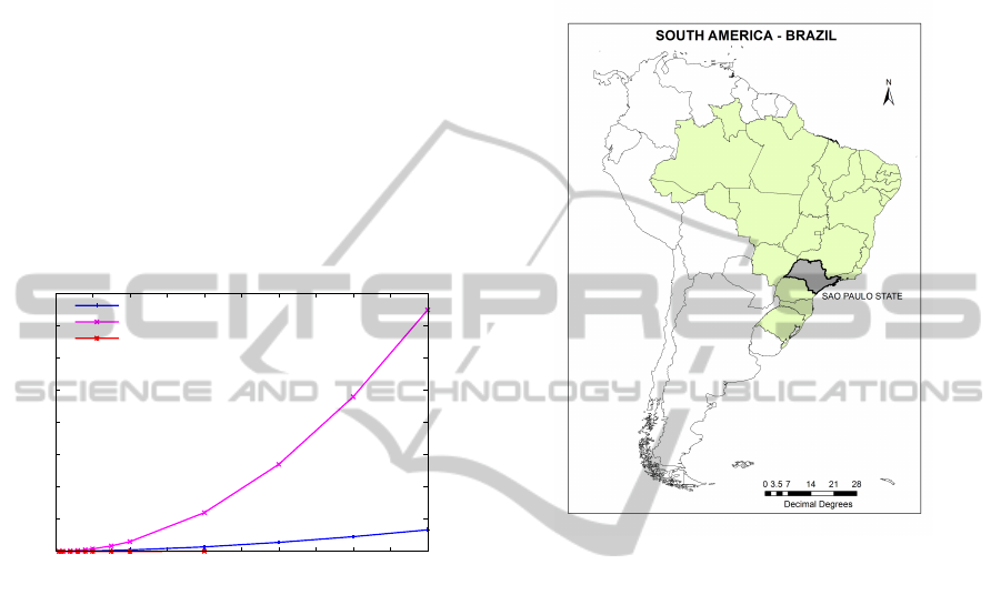
proach. For time series of length below 10, 000, both

Random Projection and the TrieMotif had a simi-

lar performance. However, as the time series length

grows, the TrieMotif presented a better performance.

This result is due to the fact that TrieMotif selects

only the candidates that are probably a match of a

motif, reducing the number of unnecessary distance

calculations. It is also possible to notice a better per-

formance of the TrieMotif using the SAX representa-

tion. The TrieMotif also consumes less memory than

the Random Projection, since the Random Projection

algorithm needs at least m

memory for the collision

matrix. From Figure 11, we can see that the memory

requirements of our method is signiﬁcantly less de-

manding than Random Projection, requiring 10 times

less memory than the state of the art (the Random Pro-

jection approach).

0 10 20 30 40 50 60 70 80 90 100

Memory Usage (GB)

Time Series Length (x1000)

TrieMotif

Random Projection

Brute-force

Figure 11: Comparison of maximum memory usage of the

TrieMotif and Random Projection.

5 REAL DATA EXPERIMENTS

We also performed experiments using data from real

applications. For this evaluation, we extracted data

from time series of remote sensing images gathered

by AVHRR/ NOAA satellite (Advanced Very High

Resolution Radiometer/National Oceanic and Atmo-

spheric Administration). These images correspond to

monthly measures of the Normalized Difference Veg-

etation Index (NDVI), which indicates the soil vegeta-

tive vigor represented in the pixels of the images and

is strongly correlated with biomass. We used images

of the S

ao Paulo state, Brazil (Figure 12), correspond-

ing to the period between April 2001 and March 2010.

From these images, we extracted 174,034 time series

of size 108. Each time series corresponds to a pair of

latitude and longitude of the S

ao Paulo state, exclud-

ing the coastal region. In order to ﬁnd the motifs in

a time series database, we created a longer time se-

ries by concatenating all time series. The TrieMotif

algorithm was created using this longer time series. It

is important to highlight that in the subsequence ex-

traction, on the ﬁrst stage, we avoided creating subse-

quences containing parts of two distinct time series,

that is, the end of a time series concatenated to the

beginning of the next one.

Figure 12: State of S

ao Paulo, Brazil.

The S

ao Paulo state was divided into 5 regions

of interest (Figure 13). The regions were obtained

through a clustering algorithm and the results were

analyzed by specialists in the agrometeorology and

remote sensing ﬁelds. According to them, region 1

corresponds to water and urban areas, regions 2 and

3 correspond to a mixture of crops (excluding sugar-

cane) and grassland, region 4 corresponds to sugar-

cane crops and region 5 to forest. Figure 14 shows

a summary of each region of interest and the number

of time series in each region. The S

ao Paulo state is

one of the greatest producers of sugarcane in Brazil.

In this work, we consider complete sugarcane cycles

of approximately one year, each of which starting in

April and ending in March, thus, we looked for the

top 4-Motifs of size n = 12 (annual measures). We

ran the TrieMotif algorithm using the bin discretiza-

tion with R = 1.5, w = 4, a = 4 and δ = 1. The exper-

iments were performed using the same computational

infrastructure of the synthetic data.

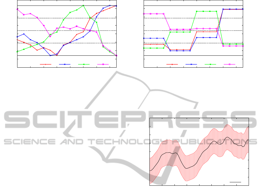
Figures 15, 16, 17, 18 and 19 show the top 4-Motif

for each region of interest. The plots are not normal-

ized due to the specialists restrictions for analyzing

them. The 1-Motif found on region 1 (Figure 15(a))

has a pattern with low values and variation, which ex-

ICEIS2014-16thInternationalConferenceonEnterpriseInformationSystems

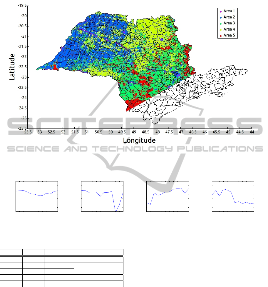
Figure 13: The S

ao Paulo state was divided into 5 regions of interest. Region 1 (purple) corresponds to water/cities, Region

2 and 3 (blue and green respectively) to a mixture of crops and grassland, Region 4 (yellow) is sugarcane crop and Region 5

(red) corresponds to forest. The black lines represent the political counties of the state. The south of the state is a forest nature

federal reserve.

-0.6

-0.4

-0.2

0.2

0.4

0.6

0.8

Mar May Jul Sep Nov Jan

NDVI

Time

(a) 1-Motif

-0.6

-0.4

-0.2

0.2

0.4

0.6

0.8

Apr Jun Aug Oct Dec Feb

NDVI

Time

(b) 2-Motif

-0.6

-0.4

-0.2

0.2

0.4

0.6

0.8

Apr Jun Aug Oct Dec Feb

NDVI

Time

-0.6

-0.4

-0.2

0.2

0.4

0.6

0.8

Dec Feb Apr Jun Aug Oct

NDVI

Time

(d) 4-Motif

Figure 15: Top 4-Motif for Region of interest 1.

Region Color # of Series Represents

1 Purple 2,804 Water and Cities

2 Blue 55,815

Grassland and

Mixture of Crops

3 Green 50,785

4 Yellow 48,301 Sugarcane crops

5 Red 16,329 Forest

Figure 14: Number of time series in each region of interest.

perts say correspond to urban regions. The other Mo-

tifs found in region 1 (Figures 15(b), 15(c) and 15(d))

have a pattern that corresponds to water regions. Fig-

ures 16 and 17 show patterns with a higher value of

NDVI and with a high variation, which specialists at-

tribute to agricultural areas.The top 3-Motifs found on

region 4 (see Figures 18(a), 18(b) and 18(c)) is clearly

recognized by agrometeorologists as a sugarcane cy-

cle, with its high values of NDVI on April and low

values on October. Since sugarcane harvesting begins

in April, the NDVI slowly starts to decrease in this

period. On October, the harvest ﬁnishes and the soil

remains exposed, thereafter the NDVI has the lowest

value. From October to March, the sugarcane grows

and the NDVI increases again. Figure 19 shows a pat-

tern with high values of NDVI and low variations, cor-

responding to the expected forest behavior, where the

NDVI follows the local temperature variation.

The TrieMotif algorithm obtained interesting re-

sults, ﬁnding patterns that were not expected by the

specialists. According to them, for some regions, the

4-Motifs found do not resemble with the expected pat-

terns. The 4-Motifs found on both regions 2 and 3

(Figures 16(d) and 17(d) respectively) indicates the

presence of sugarcane and the 4-Motif found on re-

gion 4 (Figure 18(d)) does not resemble a sugarcane

cycle. This result indicates the need for a further in-

spection in the areas where these patterns occur.

TrieMotif-ANewandEfﬁcientMethodtoMineFrequentK-MotifsfromLargeTimeSeries

0.2

0.4

0.6

0.8

Jan Mar May Jul Sep Nov

NDVI

Time

(a) 1-Motif

0.2

0.4

0.6

0.8

Sep Nov Jan Mar May Jul

NDVI

Time

(b) 2-Motif

0.2

0.4

0.6

0.8

Jul Sep Nov Jan Mar May

NDVI

Time

0.2

0.4

0.6

0.8

May Jul Sep Nov Jan Mar

NDVI

Time

(d) 4-Motif

Figure 16: Top 4-Motif for Region of interest 2.

0.2

0.4

0.6

0.8

Dec Feb Apr Jun Aug Oct

NDVI

Time

(a) 1-Motif

0.2

0.4

0.6

0.8

Jun Aug Oct Dec Feb Apr

NDVI

Time

(b) 2-Motif

0.2

0.4

0.6

0.8

Aug Oct Dec Feb Apr Jun

NDVI

Time

0.2

0.4

0.6

0.8

Apr Jun Aug Oct Dec Feb

NDVI

Time

(d) 4-Motif

Figure 17: Top 4-Motif for Region of interest 3.

0.2

0.4

0.6

0.8

Dec Feb Apr Jun Aug Oct

Time

(a) 1-Motif

0.2

0.4

0.6

0.8

Apr Jun Aug Oct Dec Feb

NDVI

Time

(b) 2-Motif

0.2

0.4

0.6

0.8

Aug Oct Dec Feb Apr Jun

NDVI

Time

0.2

0.4

0.6

0.8

Jun Aug Oct Dec Feb Apr

NDVI

Time

(d) 4-Motif

Figure 18: Top 4-Motif for Region of interest 4.

0.2

0.4

0.6

0.8

Jun Aug Oct Dec Feb Apr

NDVI

Time

(a) 1-Motif

0.2

0.4

0.6

0.8

Jan Mar May Jul Sep Nov

NDVI

Time

(b) 2-Motif

0.2

0.4

0.6

0.8

Oct Dec Feb Apr Jun Aug

NDVI

Time

0.2

0.4

0.6

0.8

Jan Mar May Jul Sep Nov

NDVI

Time

(d) 4-Motif

Figure 19: Top 4-Motif for Region of interest 5.

6 CONCLUSIONS

Finding patterns in time series is highly relevant for

applications where both the antecedent and the con-

sequent events are recorded as time series. This is the

case of climate and agrometeorological data, where

it is known that the next state of the atmosphere de-

pends in large amount of its previous state. Today,

a large network of sensing devices, such as satellites

recording both earth and solar activities, as well as

ground-based whether monitoring stations keep track

of climate evolution. However, the large amount of

data and their diversity makes it hard to discover com-

plex patterns able to support more robust analyzes. In

this scenario, is is very important to have powerful

and fast algorithms to help analyzing the that data.

In this paper we proposed TrieMotif, a novel tech-

nique that provides, in an integrated framework, an

automated technique to extract frequent patterns in

time series as K-Motifs. It reduces the resolution of

the data, speeding up the sub-sequence comparison

operations, indexes them in a trie structure and adopts

heuristics commonly employed by the meteorologists

to prune from the similarity search operations those

branches that do not represent interesting answers. In

this way, our technique is able to select only candidate

subsequences that have high probability to match a

motif, thus, reducing the number of comparisons per-

ICEIS2014-16thInternationalConferenceonEnterpriseInformationSystems

formed.

Experiments performed over data from both syn-

thetic and real applications showed that our technique

indeed perform in average 3 times faster them the

state of the art approach (Random Projection), includ-

ing the best methods previously available. It also re-

quires less memory, and the experiments revealed that

it requires up to 10 times less memory than the com-

petitor methods. We presented the results to special-

ists in the ﬁeld (meteorologists), that conﬁrmed that

the results are indeed correct and useful for their day-

to-day activities to process climate data. For future

works, we intend to explore data from larger regions,

as the whole Brazil and South America. We also in-

tend to explore data from different sensors in order to

evaluate improvements that may be needed.

ACKNOWLEDGEMENTS

The authors are grateful for the ﬁnancial support

granted by FAPESP, CNPq, CAPES, SticAmsud, Em-

brapa Agricultural Informatics, Cepagri/Unicamp and

Agritempo for data.

REFERENCES

Catalano, J., Armstrong, T., and Oates, T. (2006). Dis-

covering Patterns in Real-Valued Time Series. In

urnkranz, J., Scheffer, T., and Spiliopoulou, M., ed-

itors, Knowledge Discovery in Databases: PKDD

2006, volume 4213 of Lecture Notes in Computer Sci-

ence, pages 462–469. Springer Berlin Heidelberg.

Chiu, B., Keogh, E., and Lonardi, S. (2003). Probabilis-

tic discovery of time series motifs. In Proceedings

of the ninth ACM SIGKDD international conference

on Knowledge discovery and data mining, KDD ’03,

pages 493–498, New York, NY, USA. ACM.

Faloutsos, C., Ranganathan, M., Manolopoulos, Y., and

Manolopoulos, Y. (1994). Fast subsequence match-

ing in time-series databases. In Proceedings of the

ACM SIGMOD International Conference on Manage-

ment of Data, pages 419–429, Minneapolis, USA.

Goldin, D. Q., Kanellakis, P. C., and Kanellakis, P. C.

(1995). On similarity queries for time-series data:

Constraint speciﬁcation and implementation. In Pro-

ceedings of the 1st International Conference on Prin-

ciples and Practice of Constraint Programming, pages

137–153, Cassis, France.

Keogh, E., Chakrabarti, K., Pazzani, M., and Mehrotra, S.

(2001). Dimensionality reduction for fast similarity

search in large time series databases. Knowledge and

Information Systems, 3:263–286.

Keogh, E. and Kasetty, S. (2003). On the need for time

series data mining benchmarks: a survey and empir-

ical demonstration. In Data Mining and Knowledge

Discovery, volume 7, pages 349–371. Springer.

Keogh, E., Lin, J., Lee, S.-H., and Herle, H. (2007). Find-

ing the most unusual time series subsequence: algo-

rithms and applications. Knowledge and Information

Systems, 11(1):1–27.

Li, Y. and Lin, J. (2010). Approximate variable-length

time series motif discovery using grammar inference.

In Proceedings of the Tenth International Workshop

on Multimedia Data Mining, MDMKDD ’10, pages

10:1—-10:9, New York, NY, USA. ACM.

Li, Y., Lin, J., and Oates, T. (2012). Visualizing Variable-

Length Time Series Motifs. In SDM, pages 895–906.

SIAM / Omnipress.

Lin, J., Keogh, E., Lonardi, S., and Chiu, B. (2003). A sym-

bolic representation of time series, with implications

for streaming algorithms. In Proceedings of the 8th

ACM SIGMOD workshop on Research issues in data

mining and knowledge discovery, DMKD ’03, pages

2–11, New York, NY, USA. ACM.

Lin, J., Keogh, E., Patel, P., and Lonardi, S. (2002). Finding

motifs in time series. In In the 2nd Workshop on Tem-

poral Data Mining, at the 8th ACM SIGKDD Interna-

tional Conference on Knowledge Discovery and Data

Mining, International Conference on Knowledge Dis-

covery and Data Mining, Edmonton, Alberta, Canada.

ACM.

Lin, J., Keogh, E. J., Wei, L., and Lonardi, S. (2007). Ex-

periencing sax: a novel symbolic representation of

time series. Data Mining and Knowledge Discovery,

15:107–144.

Mohammad, Y. and Nishida, T. (2009). Constrained Motif

Discovery in Time Series. New Generation Comput-

ing, 27(4):319–346.

Rouse, J. W., Haas, R. H., Schell, J. A., and Deering, D. W.

(1973). Monitoring vegetation systems in the great

plains with ERTS. In Proceedings of the Third ERTS

Symposium, pages 309–317, Washington, DC, USA.

Udechukwu, A., Barker, K., and Alhajj, R. (2004). Discov-

ering all frequent trends in time series. In Proceedings

of the winter international synposium on Information

and communication technologies, WISICT ’04, pages

1–6. Trinity College Dublin.

Wang, L., Chng, E. S., and Li, H. (2010). A tree-

construction search approach for multivariate time se-

ries motifs discovery. Pattern Recognition Letters,

31(9):869–875.

Yankov, D., Keogh, E., Medina, J., Chiu, B., and Zordan,

V. (2007). Detecting time series motifs under uniform

scaling. In Proceedings of the 13th ACM SIGKDD

international conference on Knowledge discovery and

data mining, KDD ’07, pages 844–853, New York,

NY, USA. ACM.

TrieMotif-ANewandEfﬁcientMethodtoMineFrequentK-MotifsfromLargeTimeSeries