TV Minimization of Direct Algebraic Method of Optical Flow Detection
Via Modulated Integral Imaging using Correlation Image Sensor
Toru Kurihara and Shigeru Ando
Graduate school of Information Science and Technology, University of Tokyo, 7-3-1 Hongo, Bunkyo-ku, Tokyo, Japan
Keywords:
Optical Flow Estimation, Weighted Integral Method, Correlation Image Sensor, Total Variation.
Abstract:
A novel mathematical method and a sensing system that detects velocity vector distribution on an optical
image with a pixel-wise spatial resolution and a frame-wise temporal resolution is extended by total variation
minimization. We applied fast total variation minimization technique for exact algebraic method of optical
flow detection. Simulation result showed that directional error caused by local aperture problem decreased
effectively by the virtue of global optimization. Experimental results showed edge preserving characteristics
on the boundary of motion.
1 INTRODUCTION
Total variation (TV) minimization problem intro-
duced by Rudin et. al. has the advantage of pre-
serving edge so that applied to image analysis(Rudin
et al., 1992). Chambolle developed fast algorithm
with proof of convergence(Chambolle, 2004). Re-
cently, Zach applied TV minimization to optical flow
estimation (Zach et al., 2007).
Velocity field in the image can be considered to
be almost uniform and smooth in the object region
regardless of its texture. For example, egomotion is
approximated as quadratic function of x and y. Both
sides of the border has independent velocity fields so
that there is clear edge on the border. TV regular-
ization has desirable characteristic of smoothing con-
straint and edge preserving for optical flow estima-
tion.
Ando et. al. applied correlation image sen-
sor(Ando and Kimachi, 2003) and weighted integral
method(Ando and Nara, 2009) to optical flow estima-
tion(Ando et al., 2009). They started from optical
flow partial differential equation(Horn and Schunk,
1981) and formulated exposure time in integral form
and developed a sensing system that detects velocity
vector distribution on an optical image with a pixel-
wise spatial resolution and a frame-wise temporal res-
olution. Kurihara et. al. implemented fast optical
flow estimation algorithm achieving 3ms for 640x512
pixel resolution, and 7.5ms for 1280x1024 pixel res-
olution using GPU(Kurihara and Ando, 2013).
In this paper, we applied total variation minimiza-
tion technique for direct algebraic method of optical
flow detection using correlation image sensor. The
experimental results shows advantages of total vari-
ation regularization term, and the proposed method
successfully reconstructed smooth and edge preserv-
ing velocity fields.
2 PRINCIPLE
2.1 Correlation Image Sensor
The three-phase correlation image sensor (3PCIS) is
the two dimensional imaging device, which outputs
a time averaged intensity image g
0
(x,y) and a corre-
lation image g
ω
(x,y). The correlation image is the
pixel wise temporal correlation over one frame time
between the incident light intensity and three external
electronic reference signals.
The photo of the 640 × 512 three-phase correla-
tion image sensor is shown in Figure 1, and its pixel
structure is shown in Figure 2.
Let T be frame interval and f (x,y,t) be instant
brightness of the scene, we have intensity image
g
0
(x,y) as
g
0
(x,y) =

T /2
−T /2
f (x,y,t) dt (1)
Let the three reference signals be v
k
(t) (k = 1, 2, 3)
where v
1
(t) + v
2
(t) + v
3
(t) = 0, the resulting correla-
tion image is written like this equation.
705
Kurihara T. and Ando S..
TV Minimization of Direct Algebraic Method of Optical Flow Detection Via Modulated Integral Imaging using Correlation Image Sensor..
DOI: 10.5220/0004853207050710
In Proceedings of the 9th International Conference on Computer Vision Theory and Applications (VISAPP-2014), pages 705-710
ISBN: 978-989-758-009-3
Copyright
c
 2014 SCITEPRESS (Science and Technology Publications, Lda.)

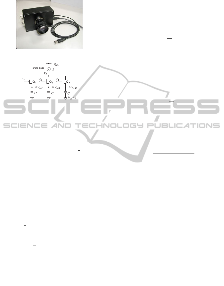
Figure 1: Photograph of Correlation Image Sen-
sor(CIS).
Figure 2: Pixel structure of the correlation image sensor.
c
k
(x,y) =

T /2
−T /2
f (x,y,t) v
k
(t)dt (2)
Here we have three reference signals with one con-
straint, so that there remains 2 DOF for the basis of
the reference signal. We usually choose orthogonal si-
nusoidal wave pair (cosωt,sin ωt) as the basis, which
means v
1
(t) = cos ωt,v
2
(t) = cos(ωt +
2
3
π),v
3
(t) =
cos(ωt +
4
3
π).
Let the time-varying intensity in each pixel be
I(x,y,t) = A(x,y)cos(ωt + ϕ(x, y)) + B(x,y,t). (3)
Here A(x,y) and ϕ(x, y) is the amplitude and phase
of the frequency component ω, and B(x,y,t) is the
other frequency component of the intensity including
DC component. Due to the orthogonality, B(x, y,t)
doesn’t contribute in the outputs c
1
,c
2
,c
3
. There-
fore the amplitude and the phase of the frequency ω
component can be calculated as follows(Ando and Ki-
machi, 2003)
A(x,y) =
2
√
3
3

(c
1
−c
2
)
2
+ (c
2
−c
3
)
2
+ (c
3
−c
1
)
2
(4)
ϕ(x,y) = tan
−1
√
3(c
2
−c
3
)
2c
1
−c
2
−c
3
(5)
From the two basis of the reference signal
(cosnω
0
t,sin nω
0
t), we can rewrite amplitude and
phase using complex equation.
g
ω
(x,y) =

T /2
−T /2
f (x,y,t)e
−jωt
dt (6)
Here ω = 2πn/T . g
ω
(x,y) is the complex form of the
correlation image, and it is a temporal Fourier coeffi-
cient of the periodic input light intensity.
2.2 Total Variation Minimization
We review TV minimization method proposed by
Chambolle(Chambolle, 2004). Let f be observed
brightness with noise. Solve minimizing problem
min
u


Ω
|∇u|dΩ +
1
2λ

Ω
(u − f )
2
dΩ

(7)
where λ is Lagrangian multiplier. Desired denoised
brightness is the solution u.
The auxiliary variable p was introduced to repre-
sent
|∇u| = max{p ·∇u ||p| ≤ 1} (8)
Then transform the minimization problem by using p,
we obtain
min
u
max
|p|≤1


Ω
p ·∇udΩ +
1
2λ

Ω
(u − f )
2
dΩ

. (9)
Exchanging min and max and from Euler-
Lagrangian equation we obtain
u = f + λ∇ ·p. (10)
The variable p for the optimized solution is calcu-
lated by the iteration
p
n+1
=
p
n
+ τ∇( f + λ∇ ·p
n
)
1 + τ|∇( f + λ∇ ·p
n
)|
. (11)
Chambolle(Chambolle, 2004) showed convergence
condition as τ < 1/8.
2.3 Direct Algebraic Solution for
Optical Flow Detection
We consider the brightness f on the object observed
in the moving coordinate system is constant. Then we
have well-known optical flow constraint
(u∂
x
+ v∂
y
) f (x,y,t) + ∂
t
f (x,y,t) = 0 (12)
where u,v is optical flow velocity, and ∂
x
= ∂/∂
x
, ∂
y
=
∂/∂
y
, ∂
t
= ∂/∂
t
. Traditional optical flow estimation
based on the OFC obtains the unknown velocity u,v
from ∂
x
f , ∂
y
f , ∂
t
f as the observed quantities.
These days, Ando et.al proposed weighted inte-
gral method for parameter estimation method for par-
tial differential equation and applied for optical flow
estimation(Ando et al., 2009). It is based on identity
relation
(u∂
x
+ v∂
y
+ ∂
t
) f (x,y,t) = 0 ∀t ∈ [−
T
2
,
T
2
]
↔

T /2
−T /2
{
(u∂
x
+ v∂
y
+ ∂
t
) f (x,y,t)
}
w(t)dt ∀w(t).
(13)
VISAPP2014-InternationalConferenceonComputerVisionTheoryandApplications
706

The temporal integration means exposure time of an
image sensor. As the weight function w(t), we can
consider an arbitrary set of complete function. Here,
we restrict our attention to the complex exponential
function set {e
−jωt
}, ω = 2πn/T,n = 0,1,2,··· for
implementation by a correlation image sensor.
Then, evaluation of integral form of optical flow
equation using integral by parts leads to

T /2
−T /2
{(u∂
x
+ v∂
y
+ ∂
t
) f (x,y,t)e
−jωt
dt
= (u∂
x
+ v∂
y
)g
ω
(x,y) + jωg
ω
(x,y)
+

f (x,y,t)e
−jωt

T /2
−T /2
= 0
(14)
where
g
ω
(x,y) =

T /2
−T /2
f (x,y,t)e
−jωt
dt (15)
is the correlation image. The unknown variables are
u,v and difference term

f (x,y,t)e
−jωt

T /2
−T /2
between
the instantaneous images at the beginning and end of
the frame.
Letting ω = 0, we obtain another relation on the
intensity image as
(u∂
x
+ v∂
y
)g
0
(x,y) +

f (x,y,t)e
−jωt

T /2
−T /2
= 0 (16)
By using Eq.(14) and Eq.(16) for eliminating dif-
ference term

f (x,y,t)e
−jωt

T /2
−T /2
, then we obtain a
complex equation
(u∂
x
+ v∂
y
){g
ω
(x,y) −g
0
(x,y)} = −jωg
ω
(x,y).
(17)
for n = 1.
Decomposing this equation into real part and
imaginary part, we obtain matrix-vector form equa-
tion

∂
x
H ∂
y
H
∂
x
K ∂
y
K

u
v

= −

h
k

(18)
where, H = ℜ[g
ω
− g
0
], K = ℑ[g
ω
− g
0
], h =
ℜ[ jωg
ω
], k = ℑ[ jωg
ω
], and ℜ and ℑ denote the real
and the imaginary part, respectively. This matrix
equation hold in each pixel, u and v can be solved
in each pixel and every frames.
When we assume u and v are uniform in the small
region Ω, then we obtain
J =
1
2

Ω
(uH
x
+ vH
y
+ h)
2
dΩ
+
1
2

Ω
(uK
x
+ vK
y
+ k)
2
dΩ. (19)
Differentiating by u and v respectively,
∂J
∂u
= S
xx
u + S
xy
v + S
x
= 0 (20)
∂J
∂v
= S
xy
u + S
yy
v + S
y
= 0 (21)
where S
xx
=

Ω
(H
2
x
+ K
2
x
)dΩ, S
yy
=

Ω
(H
2
y
+ K
2
y
)dΩ,
S
xy
=

Ω
(H
x
H
y
+ K
x
K
y
)dΩ, S
x
=

Ω
(H
x
h + K
x
k)dΩ,
S
y
=

Ω
(H
y
h + K
y
k)dΩ.
We also obtain

S
xx
S
xy
S
xy
S
yy

u
v

= −

S
x
S
y

(22)
2.4 Total Variation Minimization of
Optical Flow Estimation
We introduce regularization term in Eq.(19). That is
to find a solution of minimization problem
J =

λ(|∇u|+ |∇v|)dΩ
+
1
2

Ω
{(uH
x
+ vH
y
+ h)
2
+ (uK
x
+ vK
y
+ k)
2
}dΩ.
(23)
To solve the above problem, we introduce auxil-
iary variables u
′
and v
′
with parameter θ,
J =

λ(|∇u|+ |∇v|)dΩ
+
1
2θ


(u −u
′
)
2
+ (v −v
′
)
2

dΩ
+
1
2


(u
′
H
x
+ v
′
H
y
+ h)
2
+ (u
′
K
x
+ v
′
K
y
+ k)
2

dΩ.
(24)
The second term means distance between u and u
′
and
between v and v
′
. When we set θ sufficiently small,
the differences between u and u
′
and between v and v
′
are expected to be sufficiently small.
We solve this minimization problem by iteration
in terms of u,v and u
′
,v
′
one after another.
1. For fixed u,v, solve
min

1
2θ


(u −u
′
)
2
+ (v −v
′
)
2

dΩ
+
1
2

(u
′
H
x
+ v
′
H
y
+ h)
2
dΩ
+
1
2

(u
′
K
x
+ v
′
K
y
+ k)
2
dΩ.

(25)
From
∂J
∂u
′
=
1
θ
(u −u
′
)(−1) + (u
′
H
x
+ v
′
H
y
+ h)H
x
+ (u
′
K
x
+ v
′
K
y
+ k)K
x
= 0 (26)
TVMinimizationofDirectAlgebraicMethodofOpticalFlowDetectionViaModulatedIntegralImagingusingCorrelation
ImageSensor.
707

we obtain matrix equation

1 + θ(H
2
x
+ K
2
x
) θ(H
x
H
y
+ K
x
K
y
)
θ(H
x
H
y
+ K
x
K
y
) 1 + θ(H
2
y
+ K
2
y
)

u
′
v
′

=

u −θ(H
x
h + K
x
k)
v −θ(H
y
h + K
y
k)

(27)
u
′
, v
′
can be solved in each pixel.
2. For fixed u
′
,v
′
, solve
min


λ(|∇u|+ |∇v|)dΩ
+
1
2θ


(u −u
′
)
2
+ (v −v
′
)
2

dΩ

. (28)
The variables u and v are independent. So we can
apply Chambolle approach in section 2.2.
From
∂J
∂u
=
1
θ
(u −u
′
),
∂J
∂u
x
= λ
∂
x
u
|∇u|
,
∂J
∂u
y
= λ
∂
y
u
|∇u|
(29)
∂J
∂v
=
1
θ
(v −v
′
),
∂J
∂v
x
= λ
∂
x
v
|∇v|
,
∂J
∂v
y
= λ
∂
y
v
|∇v|
,
(30)
we obtain
u = u
′
+ λθ∇ ·p (31)
v = v
′
+ λθ∇ ·q (32)
where p =
∇u
|∇u|
, q =
∇v
|∇v|
. The parameter p and q
are solved by iteration of
p
n+1
=
p
n
+ τ∇(u
′
+ λθ∇ ·p
n
)
1 + τ|∇(u
′
+ λθ∇ ·p
n
)|
(33)
q
n+1
=
q
n
+ τ∇(v
′
+ λθ∇ ·q
n
)
1 + τ|∇(v
′
+ λθ∇ ·q
n
)|
(34)
3 EXPERIMENTS
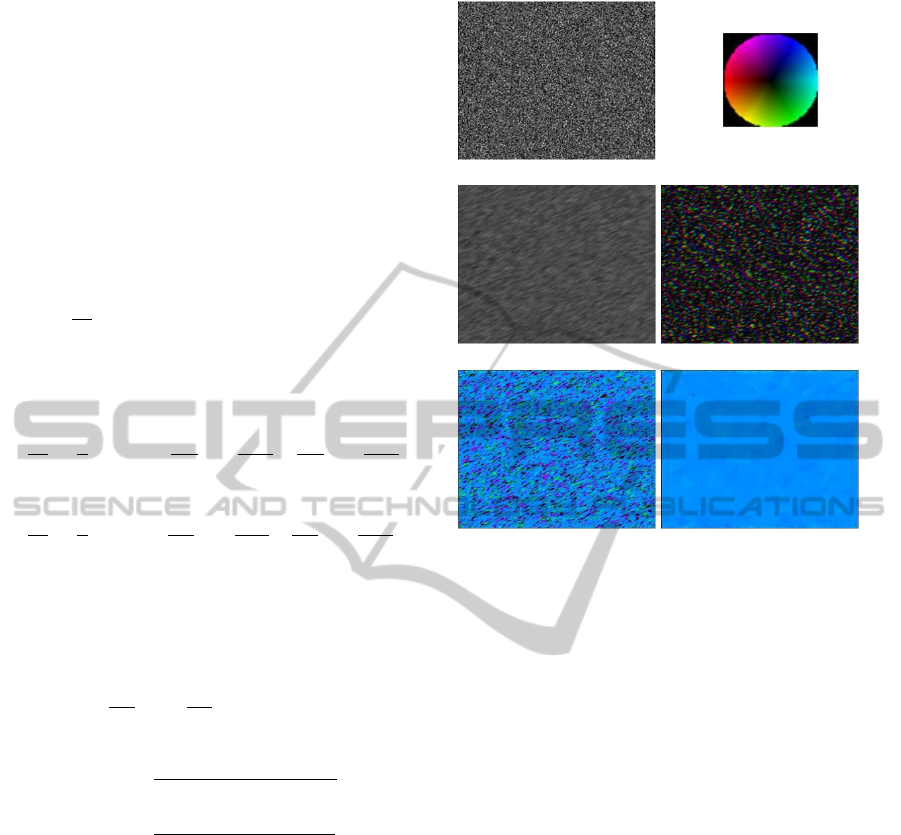
3.1 Simulation
To confirm proposed principle, we evaluate global op-
timization result. Figure 3 shows results.
By moving random dot pattern (Fig. 3(a)) in
the direction of (v
x
,v
y
) = (10.6,5.7), we compared
conventional method and TV regularization method.
Each of the result are shown in Fig. 3(e) and (f) with
the color chart of Fig. 3(b). Conventional method
shows clearly some directional error caused by aper-
ture problem. On the other hand, TV regularization
outputs global optimization results therefore the out-
put flow of each pixel is quite uniform.
(a)
(b)
(c) (d)
(e)
(f)
Figure 3: Simulation results of optical flow estima-
tion. The instantaneous pattern(a) is moved toward
v
x
= 10.6pixel/frame, v
y
= 5.7pixel/frame. Conventional
method outputs some directional error caused by aper-
ture problem. TV regularization outputs global optimiza-
tion therefore the output flow of each pixel is quite uni-
form. (a)instantaneous brightness, (b)color chart of ve-
locity representation, (c)intensity image, (d)correlation im-
age(amplitude and phase is shown by brightness and hue,
respectively.) (e)conventional method, (f)result of total
variation optimization.
3.2 Real Images on the Moving Vehicle
To confirm effect of proposed method, we compared
proposed method to conventional method by using
real images captured from the moving vehicle.
The results are shown in Fig. 4- 7. In the
Fig. 4, the output of the correlation image sensor
from the parking car is shown. In the result of con-
ventional method, there are lots of black region on
the building wall and on the vehicle moving left to
right. This is caused by textureless area. Horn &
Shunk method with modification for correlation im-
ages shows smoothing effect on the motion field re-
sulting blurred edge on the motion boundaries, but
fills black region depending on number of iterations.
Opposing to that, in the proposed method, there are
smooth velocity field on the frontal wall, and velocity
boundary on the edge of the car is successfully recon-
structed.
VISAPP2014-InternationalConferenceonComputerVisionTheoryandApplications
708

(a) Intensity image.
(b) Correlation image.
Figure 4: Example of output images of the correlation im-
age sensor. (b)correlation image only captures the area of
brightness changes, which is moving object in this example.
(a) Conventional method.
(b) Horn & Shunk method.
(c)Proposed method.
Figure 5: Optical flow of Fig. 4. In the result of conven-
tional method, there are lots of black region on the object.
Opposing to that, in the proposed method, there are smooth
velocity field on the object.
(a) Intensity image
(b) Conventional method
(c) Horn & Shunk method
(d) Proposed method
Figure 6: Result of optical flow estimation for on-vehicle
moving images. Each color represents optical flow speed
and direction by the chart in Fig. 3(b). In the result of
conventional method, there are lots of black region on the
building and vehicle moving left to right caused by texture-
less area. Opposing to that, in the proposed method, there
are smooth velocity field on the frontal wall, and veloc-
ity boundary on the edge of the car is successfully recon-
structed.
TVMinimizationofDirectAlgebraicMethodofOpticalFlowDetectionViaModulatedIntegralImagingusingCorrelation
ImageSensor.
709

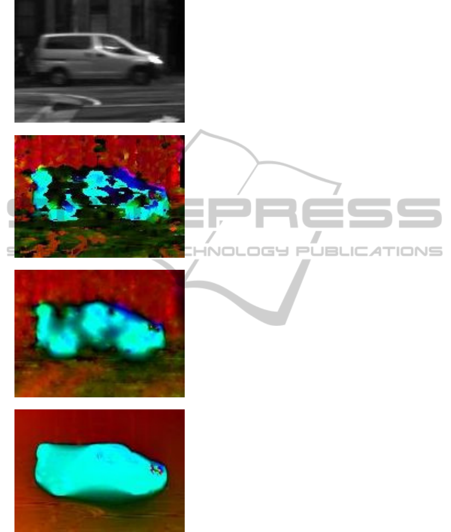
(a) Intensity image
(b) Conventional method
(c) Horn & Shunk method
(d) Proposed method
Figure 7: Center of the result in Fig. 6. In the conven-
tional method(b), there are lots of uncalculated region in
the uniform intensity area. Horn & Shunk method modi-
fied for correlation image(c) also shows uncalculated region
and blurred edge on the motion boundaries. But in pro-
posed method(d), the result shows embedded smooth flow
region in the internal area of the vehicle with preserving
flow boundary on the vehicle edge.
4 CONCLUSIONS
A novel sensing scheme and algorithm for optical
flow detection with maximal spatio and temporal res-
olution was proposed with the conjunction of Total
variation optimization scheme. It can outputs edge
preserving flow under global optimization, which
is suitable for optical flow analysis, especially for
textureless region or flow boundary of the object
edge. An experimental system was constructed with
a 640 512 pixel 3PCIS and showed good results for
moving vehicle images.
REFERENCES
Ando, S. and Kimachi, A. (2003). Correlation image sen-
sor: Two-dimensinal matched detection of amplitude-
modulated light. volume 50, pages 2059–2066.
Ando, S., Kurihara, T., and Wei, D. (2009). Exact alge-
braic method of optical flow detection via modulated
integral imaging –theoretical formulation and real-
time implementation using correlation image sensor–.
pages 480–487.
Ando, S. and Nara, T. (2009). An exact direct method
of sinusoidal parameter estimation derived from finite
fourier integral of differential equation. volume 57,
pages 3317–3329.
Chambolle, A. (2004). An algorithm for total variation
minization and applications. volume 20, pages 89–97.
Horn, B. K. P. and Schunk, B. G. (1981). Determining op-
tical flow. volume 17, pages 185–203.
Kurihara, T. and Ando, S. (2013). Fast optical flow detec-
tion based on weighted integral method using corre-
lation image sensor and gpu(in japanese). volume 3,
pages 170–171.
Rudin, L. I., Osher, S., and Fatemi, E. (1992). Nonlinear
total variation based noise removal algorithms. vol-
ume 60, pages 259–268.
Zach, C., Pock, T., and Bishop, H. (2007). A duality based
approach for realtime tv-l1 optical flow. pages 214–
223.
VISAPP2014-InternationalConferenceonComputerVisionTheoryandApplications
710