
Level Set Trees with Enhanced Marginal Density Visualization
Ky¨osti Karttunen
1
, Lasse Holmstr¨om
2
and Jussi Klemel¨a
2
1
CEMIS-Oulu, Kajaani University Consortium, University of Oulu, Kajaani, Finland
2
Department of Mathematical Sciences, University of Oulu, Oulu, Finland
Keywords:
Explorative Data Analysis, Flow Cytometry, Kernel Density Estimation, Level Set Tree, Marginal Density,
Mode Detection.
Abstract:
We study level set tree methods to analyze and visualize multivariate data. The probability density function of
the underlying distribution is estimated using a kernel density estimator, and the density estimate is visualized
using level set trees. These trees can be used to analyze the mode structure of a function. We show how level
set trees can be used to enhance more traditional density function visualization tools, like marginal densities
and slices of the density. The method is applied to flow cytometry data.
1 INTRODUCTION
Human conception of the surrounding world is effec-
tively restricted to three dimensions. In the presen-
tation of data we generally use only one or two di-
mensional (2D) structures for visualization, despite
the existing but usually unusable 3D and 4D virtual
reality environments.
Numerous methods have been developed to vi-
sualize multidimensional data, e.g. graphical ma-
trices (Bertin, 1981), parallel coordinate plots (In-
selberg, 1985), Andrew’s curves, faces, the self-
organizing map (SOM) (Kohonen, 1982; Vesanto,
1999), and scatter plots combined with projection
pursuit and multidimensional scaling. The first
decade of the personal computer age brought many
of these methods into wider use. For an overview of
these methods, see Klemel¨a (2009b, Chap. 1).
In this article we develop and apply a visualization
method that is based on level set trees, introduced in
(Klemel¨a, 2004). This visualization method can be
applied to data that are sampled from a continuous
distribution. First, the probability density function of
the observations is estimated, and then the level set
tree based tools are applied to the density estimate.
Density estimation based visualizations are an indi-
rect way to visualize data, but they have at least two
advantages: they are directly linked to making statis-
tical inference about the underlying distribution, and
they avoid the “curse of black ink”, over-plotting re-
sulting from displaying of large numbers of graphical
elements.
Indeed, methods which represent every single ob-
servation with a graphical object, like scatter plots
and parallel coordinate plots (PCP), cannot visualize a
large number of observations without filling the paper
or the computer screen. This can be avoided by using
smoothing to estimate the underlying density. For ex-
ample, in Fig. 2a a histogram density estimate is used
instead of a scatter plot. For parallel coordinate plots,
smoothing methods have been developed (Miller and
Wegman, 1991) and density based plots are reviewed
by Moustafa (2011). Alternatively,random subsetting
can be used to avoid the “curse of black ink”.
The density function of d-dimensional data is a
d-dimensional function f : R
d
→ R. Typically, mul-
tivariate density estimates are visualized using one-
and two-dimensional marginal densities and slices
(e.g. Scott, 1992). However,such visualization can be
difficult. Marginal densities suffer from the problem
that some features, for example modes, are sometimes
masked in all one- and two-dimensional marginal
densities. Slices suffer from the problem that we need
a large number of them to visualize the complete mul-
tivariate density, and it is difficult to infer the features
of the multivariate density from a large collection of
one- and two dimensional slices.
Instead of marginal densities and slices we pro-
pose to use a level set tree (LST) based methodology.
With the level set tree methods we can transform the
multivariate density to a univariate density so that cer-
tain features remain invariant.
We are particularly interested in the modes of the
density. Therefore we utilize a voluplot, which is
210
Karttunen K., Holmström L. and Klemelä J..
Level Set Trees with Enhanced Marginal Density Visualization.
DOI: 10.5220/0004844302100217
In Proceedings of the 5th International Conference on Information Visualization Theory and Applications (IVAPP-2014), pages 210-217
ISBN: 978-989-758-005-5
Copyright
c
2014 SCITEPRESS (Science and Technology Publications, Lda.)

a plot of a univariate density function that has the
same mode structure as the original multivariate den-
sity function. By a mode structure we mean the num-
ber, the size, and the hierarchical tree structure of the
modes. Finding modes of a density function can be
applied for example in model based cluster analysis
(e.g. Hartigan, 1975).
We use also baryplots, which visualize the level
set tree by showing the locations of the modes and the
centers of mass of all separated components of level
sets. Additionally, we combine baryplots with the
plots of estimates of marginal densities, and call these
plots enhanced marginal density plots. Marginal den-
sities are of course a well-known and widely used
method and we can profit from combining it with a
method which also shows the multivariate tree struc-
ture of the underlying density.
The LST-based methods are applied to flow cy-
tometry data. Flow cytometry is an optical mea-
surement technique that is used to measure biophys-
ical and chemical characteristics of cellular parti-
cles (Melamed et al., 1994). We study the number
of modes, their sizes and hierarchical structure from
data, this time, originating from paper industry.
In Section 2, the concepts related to level set trees
are reviewed. Section 3 illustrates the method with
one- and a two-dimensional examples, and Section 4
presents the application to the flow cytometry data,
and finally, Section 5 contains a discussion.
2 LEVEL SET TREES OF
DENSITY ESTIMATES
We will first give the definition of a level set tree.
Then we describe baryplots and voluplots, as well as
point out how to combine marginal densities with the
baryplots to obtain enhanced marginal plots. For a
more precise and thorough description of these con-
cepts, see (Klemel¨a, 2004; Klemel¨a, 2009b).
Level set trees, baryplots, and voluplots are calcu-
lated from kernel density estimates. A kernel density
estimator is based on data X
1
,...,X
n
∈ R
d
, assumed to
be independent and identically distributed and origi-
nating from a common density function f : R
d
→ R.
The kernel density estimator of f is defined as
ˆ
f(x) =
1
n
n
∑
i=1
K
h
(x− X
i
), (1)
where K : R
d
→ R is the kernel function, K
h
(x) =
K(x/h)/h
d
is the scaled kernel, and h > 0 is the
smoothing parameter. We choose the kernel function
K to be the standard normal density function. For
more on kernel density estimation, see (Scott, 1992).
2.1 Level Set Tree
The level set Λ( f,λ) of a function f : R
d
→ R at level
λ ∈ R is defined as the set of those points where the
function is greater than or equal to the value λ:
Λ( f, λ) = {x ∈ R
d
: f(x) ≥ λ} . (2)
To construct a level set tree, we first choose a finite
number of levels λ
1
< ··· < λ
L
. We assume that each
level set Λ( f,λ
l
), l = 1,... ,L, is either a connected
set, or that it can be decomposed into a finite number
of connected disjoint subsets,
Λ( f, λ
l
) =
K
l
[
k=1
A
lk
, l = 1, . . . , L, (3)
where A
lk
∩ A
lm
= ∅ . The sets A
lk
cannot be fur-
ther decomposed into a union of disconnected com-
ponents.
The root of a level set tree is the level set with
the lowest level λ
1
. If this level set has many discon-
nected components, then the level set tree has many
roots. Given a node of a level set tree at level λ
l
, the
child nodes of this node are among the disconnected
parts of the level set at one step higher level λ
l+1
.
The parent-child relation holds when the set associ-
ated with a child node is a subset of the set associated
with the parent node.
The level set tree is a tree whose nodes are asso-
ciated with levels λ
l
and with the sets A
lk
. The level
set tree describes the local maxima (modes) of a den-
sity function, because the leaf nodes correspond to the
local maxima.
2.2 Baryplots, Voluplots, and Enhanced
Marginal Plots
The barycenter of set A ⊂ R
d
is defined as
barycenter(A) =
1
volume(A)
Z
A
xdx. (4)
Thus, a barycenter is a d-dimensional vector that de-
fines the center of mass of a set. A baryplot is a plot
of a level set tree that consists of d windows when
the function is defined in the d-dimensional Euclidean
space. Each window shows the positions of one coor-
dinate of the barycenters for different levels:
1. the horizontal position of a node in the ith win-
dow is equal to the ith coordinate of the barycen-
ter of the set associated with the node, where
i = 1,...,d ,
2. the vertical position of a node is equal to the level
of the set associated with the node,
LevelSetTreeswithEnhancedMarginalDensityVisualization
211
−4 −2 0 2 4
0.0 0.1 0.2 0.3 0.4 0.5
(a) Density estimates
0 2 4 6 8
0.0 0.1 0.2 0.3 0.4 0.5
M1
M2
M3
(b) Voluplot
−4 −2 0 2 4
0.0 0.1 0.2 0.3 0.4 0.5
M1
M2
M3
(c) Baryplot
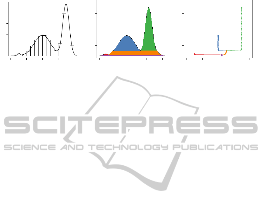
Figure 1: Panel (a) shows a kernel estimate and a histogram estimate of a 1D density with three modes. Panel (b) shows a
voluplot, and panel (c) shows a baryplot.
3. the parent–child relations are expressed by the
line joining a child with the parent.
A baryplot visualizes the “skeleton” of the func-
tion, by displaying the 1D curves that go through the
barycenters of all separated components of the level
sets. An example of a baryplot is in Fig. 1c.
A voluplot is a second type of a plot of a level set
tree. A voluplot gives information about the volumes
of the disconnected parts of the level sets. The level
set tree can be drawn in such a way that each node is
associated with a horizontal line whose length is pro-
portional to the volume of the set associated with the
node. We construct a one dimensional function whose
disconnected components of level sets are identical
with those lines, and a voluplot is a plot of this one di-
mensional function. The envelope function shown in
a voluplot is mode isomorphic with the original multi-
variate function in the sense that it has the same num-
ber of modes. The modes have the same size, and the
hierarchical tree structure of the modes is preserved.
Finally, we will consider marginal densities and
slices of a multivariate function. A one-dimensional
marginal density g : R → R of a multivariate density
function f : R
d
→ R is obtained by integrating out
d − 1 variables of f. For example,
g(x
1
) =
Z
∞
−∞
...
Z
∞
−∞
f(x
1
,x
2
,x
3
,...,x
d
) dx
2
···dx
d
.
(5)
A one-dimensional slice h : R → R of a multivariate
function f : R
d
→ R is obtained by fixing d − 1 vari-
ables to a constant value, allowing only one free vari-
able. For example,
h(x
1
) = f(x
1
,x
20
,...,x
d0
), (6)
where x
20
,...,x
d0
∈ R
d−1
are fixed. Two-dimensional
marginal densities and slices are defined analogously.
Multivariate density estimates are typically visual-
ized by calculating marginal densities and slices of the
estimates. We show below how to combine baryplots
of density estimates with estimated marginal densi-
ties.
3 EXAMPLES OF LEVEL SET
TREE PLOTS
3.1 A One Dimensional Example
LST tools were applied to visualization of one dimen-
sional data in Fig. 1. We simulated n = 40000 obser-
vations from a mixture of three normal densities. Fig-
ure 1a shows a kernel density estimate together with a
histogram density estimate. Figure 1b shows a volu-
plot, and Figure 1c shows a baryplot.
In the one dimensional case the voluplot is identi-
cal to the kernel density estimate, up to approximation
errors and a difference in the location of the functions.
The baryplot shows the level set tree together with the
locations of the modes and the barycenters.
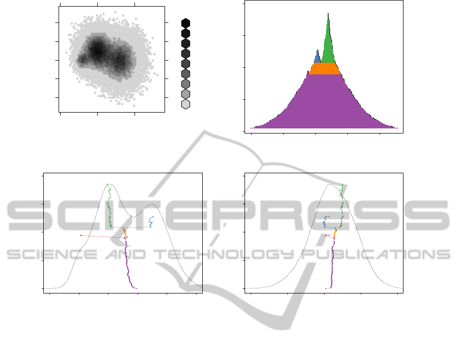
3.2 A Two Dimensional Example
Figure 2 shows an application of LST visualization to
two dimensional data. We simulated n = 10
5
obser-
vations from a mixture of three normal densities.
Panel (a) shows a histogram with a hexagonal bin-
ning. With some effort, the three modes are dis-
cernible, but their presence is not obvious. Panel (b)
shows a voluplot calculated from a kernel density es-
timate. The voluplot suggests three modes of clearly
different heights as they branch at different levels. In
the case of two modes the horizontal scale of the volu-
plot shows the distances of the modes in the original
multidimensional Euclidean space. In panels (c)-(d)
the baryplots are shown together with the marginalsof
the kernel density estimate. The labels M1, M2, and
M3 mark the modes. Note that the marginal density
IVAPP2014-InternationalConferenceonInformationVisualizationTheoryandApplications
212
dim 1
dim 2
−4
−2
0
2
4
0 5
Counts
1
41
81
120
160
200
240
279
319
359
(a) Histogram with hexagonal binning
50 60 70 80 90
0.00 0.02 0.04 0.06 0.08
M1
M2
M3
(b) Voluplot
−4 −2 0 2 4 6
0.00 0.02 0.04 0.06 0.08
M1
M2
M3
(c) Baryplot for dimension 1
−4 −2 0 2 4
0.00 0.02 0.04 0.06 0.08
M1
M2
M3
(d) Baryplot for dimension 2
Figure 2: Panel (a) shows a histogram estimate with hexagonal binning of a three modal 2D density. Panel (b) shows
a voluplot calculated form a kernel estimate, and panels (c) and (d) show the corresponding baryplots together with the
estimated marginal densities.
in panel (d) is unimodal, but the lines of the baryplot
separate the three modes.
4 FLOW CYTOMETRY DATA -
LST IN FOUR DIMENSIONS
4.1 Flow Cytometry
We analyzed laboratory data measured by a flow cy-
tometer. Flow cytometry (FCM) is an optical mea-
surement technique used typically to measure bio-
physical and chemical characteristics of thousands of
cellular particles per second. The number of mea-
sured features per particle may vary from 2 to 16, and
can be even higher in the state-of-the-art instruments.
The general objective in FCM is to sort and classify
particles (e.g. cells) into groups or clusters that can be
used in the diagnosis of disorders, such as cancer, or
HIV detection.
In addition to biomedical fields, FCM techniques
are steadily expanding into other areas, too. For ex-
ample, detection of some specific properties of wood
pulp samples by using FCM techniques has been
utilized by industrial research groups (V¨ah¨asalo and
Holmbom, 2005).
Despite the key role flow cytometers play in
biomedical organizations, FCM data are typically an-
alyzed using only two-dimensional dot or contour
plots. While other approaches, such as parallel co-
ordinate plots, can be used, the large number of par-
ticles involved restricts the usefulness of many meth-
ods. Still, careful and multifaceted inspection of FCM
data is essential to maximize the information derived
from the measurements.
4.2 Exploration of FCM data
Our FCM data originate from pulp and paper industry.
Skipping the details of the arrangement and the prac-
tical relevance in the application, the measured pulp
sample consisted of a mixture of irregular and round
particles of different composition, such as fines (cut
or crushed fibers) and pitch particles (resin). Further-
more, calibration particles of known diameter were
LevelSetTreeswithEnhancedMarginalDensityVisualization
213
FSC
SSC
FL2
FL3
X
Y
M1
M2
M3
M4
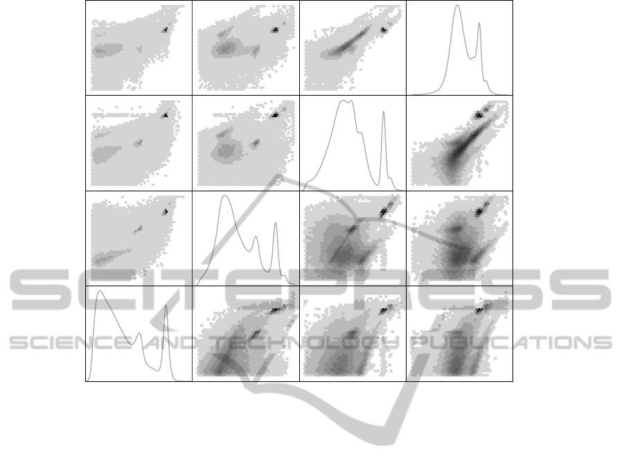
Figure 3: Scatterplot matrix and marginal densities of four dimensional FCM data are shown. Upper left pairs show linear
density (gray) scale. In lower right pairs the density scale is square root, strongly emphasizing lower densities. Note that the
data fill each graph since empty regions were left out. The M-annotations of the modes in one panel refer to Fig. 4.
added to the sample. The mean diameters of the two
added monodisperse populations were 3µm and 1µm.
In our data analysis we consider four flow cy-
tometry variables, also referred to as “parameters”
or “channels”, and named here FSC, SSC, FL2 and
FL3. Physical significance of the variables are for-
ward scatter, side scatter and two fluorescence chan-
nels, respectively.
4.2.1 Scatter Plot Matrix
A subsample of 161264 observations of the measured
FCM data set is shown in Fig. 3 as a scatter plot ma-
trix, where the scatter plots have hexagonal bins. The
observations with one component equal to zero were
removed from the data, which resulted in the removal
of 13% of the observations. Each variable was scaled
to have range [0,1]. The marginal kernel estimates of
the four variables are shown in the diagonal panels.
Several modes can be detected from these pair-
wise plots that suggest both wide and narrow struc-
tures in the data. However, these biplots represent
only two dimensional marginal densities and may not
be sufficient to capture all complexities in the data.
4.2.2 LST Method
Based on the particle type and physics in the measure-
ment system, the particles were anticipated to create
the following modal features in the measured data:
• calibration spheres: a narrow and dense mode in
all coordinates,
• fines: a wide mode with tails,
• pitch: a clearly wider mode than spheres, but nar-
rower than fines.
The kernel estimate, based on the FCM data, was
evaluated on a grid of 24
4
points. The estimate has
smoothing parameter h = 0.05 and the standard Gaus-
sian density as the kernel function.
The result of the subsequent LST data analysis is
presented in Fig. 4 where one voluplot panel (a) and
four baryplots, one for each dimension, are shown in
panels (d)-(g). Figure 4a shows that most of the data
are concentrated in the modes leaving much of the
space empty – a reflection of the curse of dimension-
ality already visible in our relatively low-dimensional
data set. In order to get a better idea of the modal
structure, panels (b) and (c) zoom into the relevant re-
gions revealing various types of modes: wide (M3),
IVAPP2014-InternationalConferenceonInformationVisualizationTheoryandApplications
214

0.00 0.02 0.04 0.06 0.08 0.10 0.12
0 5000 10000 15000
M1
M2
M3
M4
(a) Voluplot, large Euclidean space
0.0370 0.0375 0.0380 0.0385 0.0390 0.0395 0.0400
0 5000 10000 15000
M1
(b) Voluplot, left zoom range
0.0815 0.0820 0.0825 0.0830 0.0835 0.0840 0.0845
0 1000 3000
M2
M3
M4
(c) Voluplot, right zoom range
0.0 0.2 0.4 0.6 0.8 1.0
0 5000 10000 15000
(d) *FSC* coordinate: 1
M1
M2
M3
M4
0.0 0.2 0.4 0.6 0.8 1.0
0 5000 10000 15000
(e) *SSC* coordinate: 2
M1
M2
M3
M4
0.0 0.2 0.4 0.6 0.8 1.0
0 5000 10000 15000
(f) *FL2* coordinate: 3
M1
M2
M3
M4
0.0 0.2 0.4 0.6 0.8 1.0
0 5000 10000 15000
(g) *FL3* coordinate: 4
M1
M2
M3
M4
Figure 4: Four dimensional FCM data is visualized by LST voluplots and baryplots. Panel (a) shows the complete voluplot,
and panels (b) and (c) zoom into details. Panels (d)-(g) show the four baryplots, one for each coordinate, together with the
estimated marginal densities.
Figure 5: Density based parallel coordinate plot of the FCM data. The modes M1 to M4 are labeled to correspond to the ones
in Fig. 4.
LevelSetTreeswithEnhancedMarginalDensityVisualization
215

narrow (M1, M4), low (M2, M3, M4), high (M1),
all describing salient features of the four dimensional
FCM data. These 4D modes are marked in one 2D
marginal biplot in Fig. 3. To a varying degree, these
modes are visible also in other biplots but the voluplot
representation is much clearer.
A more detailed view of the modes and their posi-
tions is provided by the four baryplots in Figs. 4d–
g. As in the voluplot, the highest level set M1 is
easily identified. We may conclude that this nearly
symmetric and narrow mode actually corresponds to
the monodisperse 3 µm calibration particle popula-
tion. Symmetry and relative narrowness indicate that
the optomechanical measurement settings in the FCM
unit functioned well. Likewise, the narrow, smaller
mode M4 can be identified as the 1 µm calibration
particle population.
The wide mode M3 (see Fig. 4c) clearly represents
fines, and the slightly narrower M2 is caused by pitch.
The skewness of M2 and M3 can be observed both
from the scatterplot matrix and from the baryplots,
but the baryplots quantify the degree and direction of
skewness better.
Finally, the marginal densities added to the bary-
plots in Figs. 4d–g complement the LST plots in use-
ful way, facilitating the interpretation of baryplots.
4.2.3 Density based Parallel Coordinate Plot
To compare the LST method with a more familiar
multivariate visualization, we also created a density-
based parallel coordinate plot of the FCM data
(Fig. 5) as defined in Miller and Wegman (1991).
The kernel density estimator was used with the stan-
dard Gaussian kernel and smoothing parameter h =
0.0012. We calculated 3000 univariate estimates, and
evaluated each estimate on an equispaced grid of 1000
points. A subsample of 100000 observations was
used in the density plot.
In Fig. 5 the narrow modes M1, M2, and M4 can
be distinguished and associated with the correspond-
ing modes in Fig. 4. However, the wide mode M3,
which is clearly apparent in the LST plots, is not eas-
ily observed in the PC plot. M3 appears as a smoothly
varying background in the density-based PCP.
On the other hand, PCP suggests a mode Mx not
reported in the LST analysis. Still, Mx can be visually
observed in the enhanced baryplots as a shoulder of
the marginal near M1, although not as a mode. This
borderline case is due to the limited spatial resolution
in the 4D density and level set calculations. At the
same time it brings out issues in the LST visualization
scheme that need to be addressed in future research,
namely the need for efficient partitioning of the space
as dimension increases.
Density based PCP nicely shows the connections
of the modes in different dimensions. However, the
structure of the modes, volume, shape, skewness, kur-
tosis, etc., cannot be observed as clearly as in the LST
plots. In addition, the order of variables in the PCP
may bias the inference to some extent as opposed to
the equal treatment of the variables in the LST plots.
5 DISCUSSION
We have applied level set tree based methods to 4D
flow cytometry data. In the four dimensional case
it is possible to estimate density functions quite ac-
curately, while the more traditional methods using
marginal densities and slices are already difficult to
use in this setting, and the difficulties would rapidly
multiply if higher dimensional data were considered.
5.1 Observations – 2D or 4D
For our data, the modes can be detected both with the
scatter plot matrix (2D) and with the LST plots (4D).
However, the information provided by these methods
is different. The scatter plot matrix is based on the
histogram estimates of the two dimensional marginal
densities, whereas the LST plots are based on the ker-
nel estimates of the four dimensional density. Thus,
the LST plots visualize the concentration of the prob-
ability mass in the 4D space instead of visualizing the
concentration of the probability mass through projec-
tions to the 2D space, as is done in the scatter plot
matrix. The existence and the location of the modes
can be seen in the scatter plot matrix but the LST plots
show estimates of the full mode structure of the un-
derlying density. This means that we see estimates
of the size of the modes and estimates on the spread
of the probability mass associated with the modes.
The scatter plots give indications of these properties,
but since they show data projected to two dimensions
(estimates of 2D marginal densities), we cannot in-
fer the size of the modes and the spread of the prob-
ability mass in the 4D space. In FCM data analy-
sis, the LST methods can simultaneously identify and
quantify features of multidimensional particle clusters
from large and dominating modes down to small and
easily missed concentrations. This feature may prove
to be highly valuable for example in medical FCM
data exploration.
There are examples where the modes can be de-
tected with the LST plots but not with the scatter
plot matrices. This can happen when the modes are
so close to each other that they mask each other in
projections, see Klemel¨a (2004). On the other hand,
IVAPP2014-InternationalConferenceonInformationVisualizationTheoryandApplications
216

scatter plot matrices may in some cases detect modes
where the LST plots fail. This may happen when
the number of variables (dimension of the observa-
tions) is so large that density estimation becomes in-
tractable.
5.2 Clustering
Scatter plot matrices and parallel coordinates plots are
not model based clustering methods. They need to
be accompanied with a separate statistical technique
to provide estimates and confidence statements about
the mode structure. Mode detection with LST plots
is an example of model based clustering. A voluplot
gives an estimate of the so called excess mass of a
mode. In our future work we plan to use this to as-
sociate statistical significance to the modes suggested
by LST plots.
5.3 Finally
To conclude, the combination of voluplots and bary-
plots with marginal densities offers promising en-
hancements to more traditional visualizations and
deepens the insight into the otherwise hidden multi-
dimensional structures in data.
ACKNOWLEDGEMENTS
In addition to the R-code written by the authors, sev-
eral R-packages were utilized (R Core Team, 2012;
Sarkar, 2008; Klemel¨a, 2009a; Carr, 2011; Lemon,
2006).
This work has been partially supported by the
Academy of Finland research project 250862 and by
the Finnish Funding Agency for Technology and In-
novation (Tekes) research project 40292/12.
REFERENCES
Bertin, J. (1981). Graphics and Graphic Information-
Processing. De Gruyter, Berlin.
Carr, D. (2011). hexbin: Hexagonal binning routines. R
package, ported by Lewin-Koh, N. and Maechler M.
Inselberg, A. (1985). The plane with parallel coordinates.
The Visual Computer, 1(2):69–91.
Klemel¨a, J. (2004). Visualization of multivariate density es-
timates with level set trees. Journal of Computational
and Graphical Statistics, 13(3):599–620.
Klemel¨a, J. (2009a). denpro: Visualization of multivariate
functions, sets, and data. R package.
Klemel¨a, J. (2009b). Smoothing of Multivariate Data– Den-
sity Estimation and Visualization. Wiley, New York.
Kohonen, T. (1982). Self-organized formation of topolog-
ically correct feature maps. Biological Cybernetics,
43(1):59–69.
Lemon, J. (2006). Plotrix: R package. R-News, 6(4):8–12.
Melamed, M. R., Lindmo, T., and Mendelsohn, M. L.
(1994). Flow Cytometry and Sorting. Wiley-Liss,
New York.
Miller, J. J. and Wegman, E. J. (1991). Construction of line
densities for parallel coordinate plots. In Buja, A. and
O., T., editors, Computing and Graphics in Statistics,
pages 107–123. Springer, New York.
R Core Team (2012). R: A language and environment for
statistical computing.
Sarkar, D. (2008). Lattice: Multivariate Data Visualization
with R. Springer, New York.
Scott, D. W. (1992). Multivariate Density Estimation: The-
ory, Practice, and Visualization. Wiley, New York.
V¨ah¨asalo, L. and Holmbom, B. (2005). Influence of latex
properties on the formation of white pitch. Tappi Jour-
nal, 4(5):27–32.
Vesanto, J. (1999). Som-based data visualization methods.
Intelligent Data Analysis, 3(2):111–126.
LevelSetTreeswithEnhancedMarginalDensityVisualization
217
