SCHOG Feature for Pedestrian Detection

Ryuichi Ozaki and Kazunori Onoguchi

Graduate School of Science and Technology, Hirosaki University, 3 Bunkyo-cho, Hirosaki, Aomori, 036-8561, Japan

Keywords:

Pedestrian detection, Co-occurrence Histograms of Oriented Gradients, Similarity, Support Vector Machine.

Abstract:

Co-occurrence Histograms of Oriented Gradients(CoHOG) has succeeded in describing the detailed shape of

the object by using a co-occurrence of features. However, unlike HOG, it does not consider the difference of

gradient magnitude between the foreground and the background. In addition, the dimension of the CoHOG

feature is also very large. In this paper, we propose Similarity Co-occurrence Histogram of Oriented Gradi-

ents(SCHOG) considering the similarity and co-occurrence of features. Unlike CoHOG which quantize edge

gradient direction to eight directions, SCHOG quantize it to four directions. Therefore, the feature dimen-

sion for the co-occurrence between edge gradient direction decreases greatly. In addition to the co-occurrence

between edge gradient directions the binary code representing the similarity between features is introduced.

In this paper, we use the pixel intensity, the edge gradient magnitude and the edge gradient direction as the

similarity. In spite of reducing the resolution of the edge gradient direction, SCHOG realizes higher perfor-

mance and lower dimension than CoHOG by adding this similarity. We have focused on pedestrian detection

in this paper. However, this method is also applicable to various object recognition by introducing various

kind of similarity. In experiments using the INRIA Person Dataset, SCHOG is evaluated in comparison with

the conventional CoHOG.

1 INTRODUCTION

Recently, a pedestrian detection system have been

put to practical use as a vehicle safety device(Hattori

et al., 2009). Since features expressing characteris-

tics of a person well is important in these system,

various features for pedestrian detection have been

proposed. T.Ojala et al. proposed the Local Binary

Pattern(LBP)(Ojala et al., 1996) representing the re-

lation between the intensity of an interest pixel and

the intensity of eight adjacent pixels. This feature

has been studied in various ways because it’s robust

to illumination change and it’s implemented easily.

Y.Cao et al. proposed the Advanced LBP(Cao Yun-

yun, 2011) which is robust to noise and low inten-

sity. N.Dalal proposed HOG(Dalal and Triggs, 2005)

feature which is robust to the change of the pedes-

trian’s posture and the change of the illumination by

generating the histogram of the edge gradient ori-

entation in each block and normalizing each block

for every cell. They also proposed the feature fo-

cusing on the gradient orientation of the time se-

ries(Dalal et al., 2006). T.Watanabe et al. proposed

CoHOG feature that represented the co-occurrence of

gradient orientation and showed high performance for

pedestrian detection. As other features using the co-

occurrence, T.Kobayashi et al. proposed a Gradient

Local Auto-Correlation(GLAC)(Kobayashiand Otsu,

2008) which calculated the autocorrelation of the po-

sition and edge gradient orientation. K.Yamaguchi

et al. proposed a two-dimensional gradient orienta-

tion histogram using polar coordinates which can ex-

press small difference(K. Yamaguchi, 2011). S.Walk

et al. proposed the Color Self-Similarity(CSS)(Walk

et al., 2010) feature using the similarity of HSV his-

togram in the local area. As mentioned above, the

co-occurrence of feature is effective for improving

the performance of pedestrian detection. However,

there is a problem that the dimension of the feature

increases signiﬁcantly.

In this paper, we propose SCHOG which consists

of the co-occurrence of edge gradient direction and

the similarity. Although SCHOG quantizes edge gra-

dient direction to the half of CoHOG, it can represent

the shape of the object more ﬁnely than CoHOG by

adding the similarity to the co-occurrenceof edge gra-

dient direction. Because the similarity is represented

by the binary code, the dimension of SCHOG is a

half of the conventional CoHOG in spite of adding the

similarity. We evaluate three kind of similarity, such

as the pixel intensity, the edge gradient magnitude and

the edge gradient direction in the experiment. These

Ozaki R. and Onoguchi K..

SCHOG Feature for Pedestrian Detection.

DOI: 10.5220/0004813000600066

In Proceedings of the 3rd International Conference on Pattern Recognition Applications and Methods (ICPRAM-2014), pages 60-66

ISBN: 978-989-758-018-5

 2014 SCITEPRESS (Science and Technology Publications, Lda.)

values are not used directly in CoHOG. Therefore, the

proposed feature can compensate information lost in

CoHOG. In the experiment, the edge gradient magni-

tude showed the best performance.

Experimental result using the INRIA Person

Dataset and the Support Vector Machine shows that

the performance of SCHOG is better than the conven-

tional CoHOG.

The rest of this paper is organized as follow. In

Section 2, the proposed method is explained in detail

and its extensibility is discussed. In Section 3, the

performance of the SCHOG is evaluated by compar-

ing with the conventional CoHOG. In Section 4, this

paper is summarized.

2 PROPOSED FEATURE

Pedestrians show a various shape, e.g., standing, run-

ning, or shaking the hand. In addition, they wear

clothes of various texture and color. Moreover, in the

outdoor, illumination changes frequently and a lot of

image noise occurs. CoHOG has solved these prob-

lems to some extent although it needs very large fea-

ture dimension. The proposed feature (SCHOG) im-

proves CoHOG so that it can have better performance

and lower feature dimension.

2.1 CoHOG

In this section, the outline of CoHOG is explained.

CoHOG uses a two-dimensional histogram whose bin

is a pair of edge gradient direction between the inter-

est pixel and the offset pixel. The feature dimension

becomes large since histograms are created for every

combination of the interest pixel and the offset pixel.

However, it can represent object shape ﬁnely and it is

robust to the change of shape and illumination.

At ﬁrst, the edge gradient magnitude(M) and the

edge gradient direction(θ) are obtained from equa-

tions (1) and (2).

θ(x, y) = tan

−1

(x, y)

(1)

M(x, y) =

(x, y)

+ f

(x, y)

, (2)

where f

(x, y) and f

(x, y) denote edge gradient

magnitude of horizontal direction and that of verti-

cal direction in the pixel (x, y), which are calculated

by Sobel operator. Gradient direction(θ) is quantized

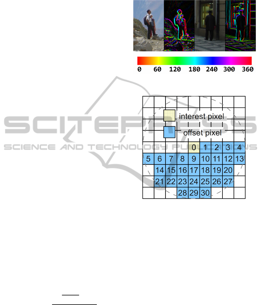
to eight directions by 45 degrees. Figure 1 shows the

gradient direction image and the gradient magnitude

image. The direction is represented by color and the

Figure 1: Examples of gradient direction and gradient mag-

nitude.

Figure 2: The number and position of the offset pixel.

magnitude is represented by the brightness. Same di-

rection often appears around the contour of a pedes-

trian. CoHOG represents this characteristic by the co-

occurrence of edge gradient direction between the in-

terest pixel and the offset pixel.

31 offset pixels are set around the interest pixel as

shown in Figure 2. The interest pixel is included in

offset pixels. Two dimensional histogram is created

for every offset pixel. If the offset pixel corresponds

the interest pixel, the histogram has eight bins because

the gradient direction of each pixel is same. Except

for this case, the histogram has 8 × 8 = 64 bins be-

cause the number of bins is a combination of gradient

direction.

The input image is divided into several rectangular

blocks as shown in Figure 3. In each block, the 2D

histogram is created for every offset pixels. Let (p, q)

be the image coordinate system whose origin is at the

upper left of each block, (x, y) be a offset coordinate

system whose origin is at the interest pixel and C

x,y

be the 2D histogram of an offset pixel (x, y). The bin

SCHOGFeatureforPedestrianDetection

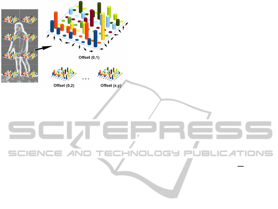
Figure 3: Example of 2D histogram in CoHOG.

x,y

(i, j) of 2D histogram C

x,y

is incremented by

x,y

(i, j)

n−1

∑

p=0

m−1

∑

q=0











if I(p, q) == i

and I(p+ x,q+ y) == j

0 otherwise ,

where I is the gradient-orientation image, n is

the horizontal size of a block and m is the vertical

size of a block. In each block, feature dimension is

8 + 64 × 30 = 1928. Figure 3 shows the example

of the 2D histogram in CoHOG. In this example,

an input image is divided into 2 × 8 blocks and in

each block, the 2D histogram is created for every

offset pixels. CoHOG does not perform the normal-

ization of the histogram because CoHOG does not

accumulate the gradient magnitude in the bin of the

histogram, unlike HOG feature.

2.2 SCHOG

Since CoHOG uses only the relation between the gra-

dient direction of the interest pixel and that of the

offset pixel, other information acquired on the way,

such as the pixel intensity or the gradient magnitude,

is thrown away. SCHOG improves the performance

by adding this information. SCHOG uses not only

the co-occurrence of the gradient direction but also

that of the similarity. In this paper, we evaluate the

pixel intensity, the gradient magnitude and the gra-

dient direction as the similarity although various fea-

tures can be use as the similarity. The computing time

does not increase because these features are obtained

as the gradient direction is calculated.

The procedure of feature extraction is described

below. At ﬁrst, the gradient intensity and the gradi-

ent orientation are calculated by equations (1) and (2)

as well as CoHOG. Offset pixels around the interest

pixel are set as the same position as CoHOG. Next,

we create the 2D histogram representing the relation

between the gradient direction of the interest pixel and

that of the offset pixel. Unlike CoHOG, the gradient

direction is quantized to four directions by 90 degrees.

However, the gradient direction is quantized to eight

directions by 45 degrees when the offset pixel cor-

responds the interest pixel because this hardly inﬂu-

ences the number of feature dimension, as described

later. The main difference between SCHOG and Co-

HOG is that SCHOG adds the similarity between fea-

tures, such as the pixel intensity, the gradient magni-

tude or the gradient orientation, to the co-occurrence

of the gradient direction. SCHOG can represent the

shape of the object more ﬁnely than CoHOG since

these features which CoHOG does not use directly

are incorporated. The similarity between the interest

pixel and the offset pixel is given by

sim1

) =











0 if T

< tan

−1

< T

1 otherwise

sim2

) =











if T

< |V

−V

or T

> |V

−V

1 otherwise ,

where F

sim1

is the similarity function for the pixel

intensity or gradient magnitude, F

sim2

is the similar-

ity function for the gradient angle, V

is the pixel in-

tensity, the gradient magnitude or the gradient direc-

tion in the intensity pixel and V

is the pixel intensity,

the gradient magnitude or the gradient direction in the

offset pixel. Thresholds T

, T

and T

in equations

(3) and (3) were determined experimentally. The sim-

ilarity returns 0 when features are similar and it re-

turns 1 when features are different. The feature di-

mension is suppressed because the similarity is repre-

sented by the binary code.

We divide the input image into 6× 12 blocks. Let

(p, q) be the image coordinate system whose origin

is at the upper left of each block, (x,y) be a offset

coordinate system whose origin is at the interest pixel

and C

x,y,s

be the histogram of an offset pixel (x, y) and

similarity s. The binC

x,y,s

(i, j, k) of histogramC

x,y,s

incremented by

ICPRAM2014-InternationalConferenceonPatternRecognitionApplicationsandMethods

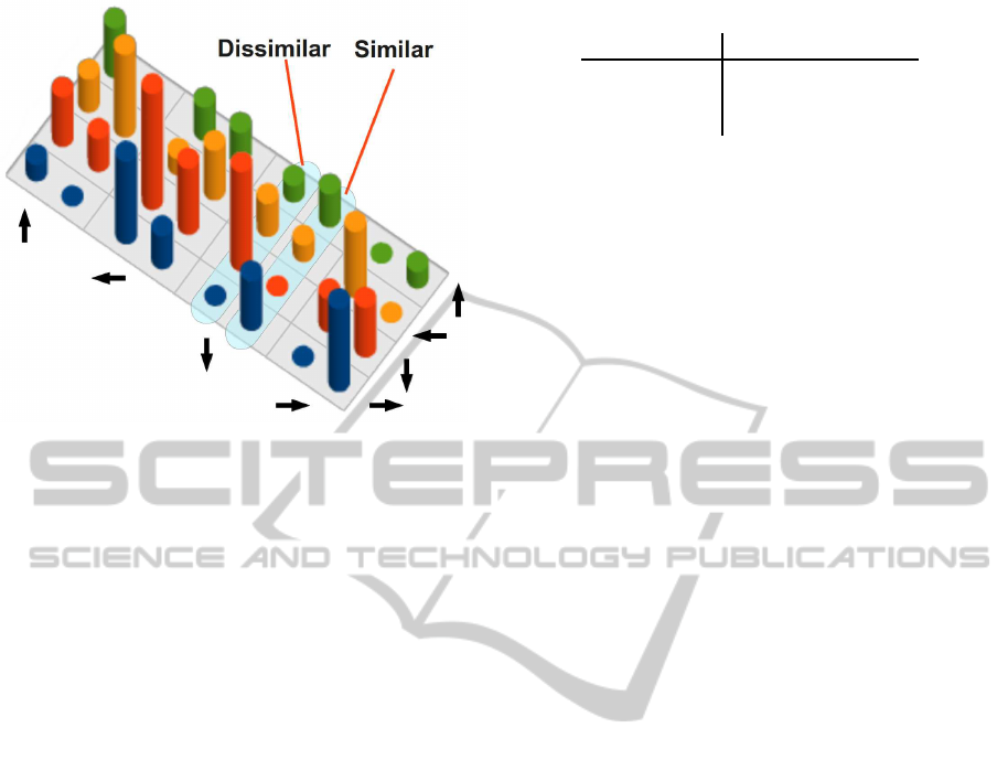
Figure 4: Example of a histogram used in SCHOG.

x,y,s

(i, j, k)

n−1

∑

p=0

m−1

∑

q=0











if I(p, q) == i

and I(p+ x, q+ y) == j

and F

sim

(a, b) == k

0 otherwise ,

Where I is gradient-orientation image, n and m

represent the size of a block, a represents feature

value at the offset pixel, b represents feature value at

the interest pixel. k(0 or 1) represents the similarity.

When the offset pixel corresponds the interest pixel,

the dimension is 8. Since this case is not related to

the co-occurrence, number of total feature dimension

hardly increase even if the dimension is 8. The other

offset pixel has 16 dimensions for a combination of 4

gradient directions and 2 dimensions for the similar-

ity. Therefore, in each block, the total dimension of

SCHOG is 8+ 16× 2× 30= 968. This is about a half

of CoHOG. Figure 4 shows the example of the his-

togram representing the co-occurrence of the gradient

direction and the gradient magnitude. There are two

bins that represent the similarity for each combination

of directions.

In this paper, we use the pixel intensity, the gra-

dient magnitude or the gradient direction as the fea-

ture for the similarity. However, the framework of

SCHOG can easily introduce various features, avoid-

ing the steep increase in a number of dimension be-

cause it uses the binary code to represent the simi-

larity. The name described in Table 1 is attached for

every kind of similarity. SCHOG-pix uses the pixel

intensity as the similarity. SCHOG-gra uses the gra-

dient magnitude as the similarity. Although this in-

formation is directly used in HOG, it is deleted in Co-

Table 1: The name of SCHOG for each similarity.

name

similarity

SCHOG-pix pixel intensity

SCHOG-gra gradient magnitude

SCHOG-ang

gradient direction

HOG. SCHOG-ang uses the gradient direction as the

similarity. Since this similarity is calculated from the

angle before quantization, it’s expected that the ﬁner

relation between gradient directions can be expressed.

3 EXPERIMENTAL RESULTS

We carried out experiments using a SVM classi-

ﬁer(SVMLight, Linear-kernel). The ROC curve,

which shows the True Positive ratio for the vertical

axis and shows the False Positive ratio for the hor-

izontal axis, is used for evaluating the performance.

It shows that performance is better, so that the curve

goes to the upper left.

3.1 Dataset

We adopted INRIA Person Dataset that various pre-

vious paper have used for evaluation. Figure 5 shows

some examples in this dataset. We used 2,416 posi-

tive images and 12,180 negative images for training.

Ten regions randomly extracted from an image were

used as negative images. The size of a positive image

is 64× 128 pixels and the size of a negative image is

from 214× 320 to 648× 486. 1,132 positive images

and 453 negative images are used for test. The size of

a positive image is as same as an image for training

and the size of a negative image is from 242× 213 to

690× 518. The dataset used in experiments is sum-

marized in Table 2.

3.2 Feature Decrease in CoHOG

Before evaluating the performance of SCHOG, we

examined how much performance decreased by quan-

tizing the gradient direction to four directions. We

names SCHOG without the similarity SCHOG-no-

sim. This is the same as CoHOG whose gradient di-

rection is quantized to not eight directions but four di-

rections. The dimension of SCHOG-no-sim is about

1/4 of CoHOG. Figure 6(a) shows the performance

of SCHOG-no-sim and CoHOG. The fall of perfor-

mance which occurred by reducing quantization of

the gradient direction is few. This result shows that

four directions are enough for the co-occurrence of

SCHOGFeatureforPedestrianDetection

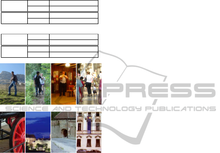
Table 2: Details of INRIA Person Dataset.

(a) Training data

image size positive 64× 128

negative 214× 320 - 648× 486

number positive 2416

negative 1218× 10 = 12180

(b) Test data

image size positive 64× 128

negative 242× 213 - 690× 518

number positive 1132

negative 453

(a) positive image

(b) negative image

Figure 5: Example of INRIA Person Dataset. (a) Person

image (b) Cropped negative.

the gradient direction if this slight fall of performance

is supplemented with other features like the similarity.

3.3 Effect of Similarity

Figure 6(b) shows the performance of CoHOG,

SCHOG-pix, SCHOG-gra and SCHOG-ang.

SCHOG-pix, SCHOG-gra and SCHOG-ang use

the pixel intensity, the gradient magnitude and the

gradient direction as the similarity respectively. The

dimension of these features is a half of CoHOG. In

Figure 6(b), the True Positive ratio of SCHOG-pix,

SCHOG-gra, SCHOG-ang and CoHOG is 90.12%,

93.13%, 87.37% and 88.07% respectively when the

False Positive ratio is 0.1%. SCHOG-pix shows

the almost same performance as CoHOG although

it uses the simple feature like the pixel intensity as

the similarity. SCHOG-gra, which uses the gradient

magnitude as the similarity, shows quite better

performance than CoHOG. This result shows that the

gradient magnitude which CoHOG omitted is effec-

tive to improve performance of pedestrian detection.

The performance of SCHOG-ang is slightly inferior

to CoHOG. This result shows that the similar feature

does not contribute to improvement in performance.

In this experiment, it was shown that SCHOG whose

similarity is the gradient magnitude can obtain better

performance than CoHOG although the resolution

of the gradient direction is a half of CoHOG. The

summary of features used in this experiment is shown

in Table 3.

Figure 7 shows failure examples of SCHOG-gra

and CoHOG. Figure 7(a) shows examples to which

both SCHOG-gra and CoHOG failed in detection.

Pedestrians with low contrast to a background were

not detected. Figure 7(b) shows examples to which

only CoHOG failed in detection. CoHOG failed be-

cause the gradient direction around a pedestrian’s

contour is scattering, but SCHOG succeeded using

the difference in the gradient magnitude between a

pedestrian and a background. Figure 7(c) shows ex-

amples to which only SCHOG failed in detection.

In these examples, pedestrians were not detected be-

cause the gradient magnitude around the pedestrian’s

contour is similar.

4 CONCLUSIONS

In this paper, we proposed the novel feature named

SCHOG which improved CoHOG feature so that the

detection performance might improve and the fea-

ture dimension might decrease. SCHOG consists of

the co-occurrence of edge gradient direction and the

similarity. Although SCHOG quantizes edge gradi-

ent direction to the half of CoHOG, it can represent

the shape of the object more ﬁnely than CoHOG by

adding the similarity to the co-occurrenceof edge gra-

dient direction. Because the similarity is represented

by the binary code, the dimension of SCHOG is a

half of the conventional CoHOG in spite of adding the

similarity. Experimental results using INRIA Person

Dataset showed that reducing quantization of the gra-

dient direction hardly causes the fall of performance

and SCHOG whose similarity is gradient magnitude

have quite better performance than CoHOG.

As the similarity, the pixel intensity, the gradi-

ent magnitude and the gradient direction were eval-

uated in this paper. However, since the similarity is

simply represented by the binary code, other various

features such as color information or a combination

of features are allowed as the similarity. Therefore,

SCHOG can be applied to various application of ob-

ject recognition. Presently, our method uses the same

ICPRAM2014-InternationalConferenceonPatternRecognitionApplicationsandMethods

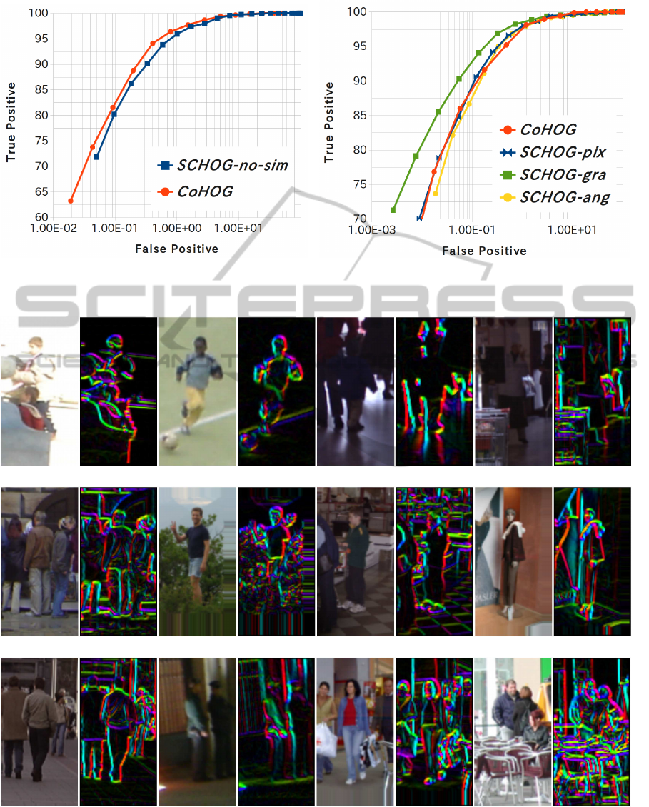
(a) Performance of CoHOG and SCHOG-no-sim. (b) Comparison of the proposed method and CoHOG.

Figure 6: Performance of the proposed method.

(a) Examples to which both CoHOG and SCHOG-gra failed in detection.

(b) Examples to which only CoHOG failed in detection.

Figure 7: Examples of failure detection. Left is the original image, and right is gradient direction image.

arrangement of offset pixels as CoOG. However, this arrangement is important for improving performance

SCHOGFeatureforPedestrianDetection

Table 3: Summary of proposed features.

Name Dimension per Block Similarity Performance TP(FP=0.1[%])

SCHOG-pix 8+ 16× 2× 30= 968 pixel intensity fair 90.1066

SCHOG-gra 8+ 16× 2× 30= 968 magnitude good 93.1310

SCHOG-ang 8+ 16× 2 × 30= 968 gradient direction bad 87.3676

CoHOG 8+ 8× 8× 30= 1928 bad 88.0733

and the number of dimension can be reduced greatly

if the number of offset pixels is reduced. In the future,

we will examine the optimal arrangement and optimal

number of offset pixels. Then, we clarify the perfor-

mance by experiments using different data sets.

REFERENCES

Cao Yunyun, H. N. (2011). Detecting pedestrians using an

advanced local binary pattern histogram. In 18th ITS

World Congress, Orlando, 2011. Proceedings.

Dalal, N. and Triggs, B. (2005). Histograms of oriented

gradients for human detection. In Schmid, C., Soatto,

S., and Tomasi, C., editors, International Conference

on Computer Vision & Pattern Recognition, volume 2,

pages 886–893, INRIA Rhˆone-Alpes, ZIRST-655, av.

de l’Europe, Montbonnot-38334.

Dalal, N., Triggs, B., and Schmid, C. (2006). Human de-

tection using oriented histograms of ﬂow and appear-

ance. In Proceedings of the 9th European conference

on Computer Vision - Volume Part II, ECCV’06, pages

428–441, Berlin, Heidelberg. Springer-Verlag.

Hattori, H., Seki, A., Nishiyama, M., and Watanabe, T.

(2009). Stereo-based pedestrian detection using mul-

tiple patterns. In BMVC. British Machine Vision As-

sociation.

K. Yamaguchi, T. N. (2011). Two dimensional histograms

of oriented gradients for pedestrian detection. IEICE

Transactions on Fundamentals of Electronics, Com-

munications and Computer Sciences. D, Information

System, 94(1):365–373.

Kobayashi, T. and Otsu, N. (2008). Image feature extrac-

tion using gradient local auto-correlations. In Forsyth,

D. A., Torr, P. H. S., and Zisserman, A., editors, ECCV

(1), volume 5302 of Lecture Notes in Computer Sci-

ence, pages 346–358. Springer.

Ojala, T., Pietik¨ainen, M., and Harwood, D. (1996). A com-

parative study of texture measures with classiﬁcation

based on featured distributions. Pattern Recognition,

29(1):51–59.

Walk, S., Majer, N., Schindler, K., and Schiele, B. (2010).

New features and insights for pedestrian detection. In

Conference on Computer Vision and Pattern Recogni-

tion (CVPR), San Francisco. IEEE, IEEE.

ICPRAM2014-InternationalConferenceonPatternRecognitionApplicationsandMethods