
A Method for Document Image Binarization based on Histogram
Matching and Repeated Contrast Enhancement
Mattias Wahde
Department of Applied Mechanics, Chalmers University of Technology, G¨oteborg, Sweden
Keywords:
Document Image Binarization, Image Processing.
Abstract:
In this paper, a new method for binarization of document images is introduced. During training, the method
stores histograms from training images (divided into small tiles), along with the optimal binarization threshold.
Training image tiles are presented in pairs, one noisy version and one clean binarized version, where the
latter is used for finding the optimal binarization threshold. During use, the method considers the tiles of an
image one by one. It matches the stored histograms to the histogram for the tile that is to be binarized. If a
sufficiently close match is found, the tile is binarized using the corresponding threshold associated with the
stored histogram. If no match is found, the contrast of the tile is slightly enhanced, and a new attempt is made.
This sequence is repeated until either a match is found, or a (rare) timeout is reached. The method has been
applied to a set of test images, and has been shown to outperform several comparable methods.
1 INTRODUCTION
The problem of identifying text in images has at-
tracted much attention in recent years, especially
with the advent of generally available, low-cost high-
quality cameras. There are many possible appli-
cations (Neumann and Matas, 2010; Gonz´alez and
Bergasa, 2013), for example reading the license plates
of vehicles, identifying labels on packaging, helping
the visually impaired to read signs and other texts etc.
An interesting special case is that of identifying and
reading text in document images, such as letters, bank
statements etc. While perhaps less difficult than iden-
tifying text in a completely general image, this case
also presents challenges and has been the subject of
much research; see e.g. (Stathis et al., 2008; Shi et al.,
2012; Valizadeh and Kabir, 2013).
As an example, automatic reading of a letter (or
some other text) held in front of a camera, is a poten-
tially useful application. Such a procedure can be in-
cluded in an intelligent agent intended for helping the
visually impaired, particularly elderly people, to man-
ange everyday tasks. Indeed, the method presented
below is intended to form a part of such a system.
Once completed, the agent, represented as a face on
a screen, and running on a computer equipped with a
microphone, a camera, and loudspeakers, will interact
with a user to aid in a variety of tasks, including (but
not limited to) the one just mentioned.
In order to read the text in a document image
using, for example, an already available OCR sys-
tem, a common first step is to binarize the image,
i.e. taking an often noisy image with varying illu-
mination levels and converting it to an image, ide-
ally containing easily identifiable black characters on
a white background. The main difficulties concern
brightness variations (due to, for example, spotlights
or bad lighting altogether), stains, misaligned text
(due to bending), and other noise sources. In re-
cent years, several binarization methods have been
suggested for document images; see e.g. (Stathis
et al., 2008; Chen et al., 2012; Shi et al., 2012;
Lu et al., 2010). In order to assess the perfor-
mance of such methods, they are often compared with
the performance of several commonly used bench-
mark methods, such as Otsu’s method (Otsu, 1979),
Niblack’s method (Niblack, 1986) and Sauvola’s
method (Sauvola and Pietik¨ainen, 2000).
In this paper, a new method for binarization will
be presented, based on histogram matching, i.e. a
comparison between the histogram of (a part of) a
document image and the histogram of a stored image
for which the optimal binarization threshold is known
as a result of a training procedure. In addition, the
proposed method employs iterative enhancement of
images in cases where no adequate histogram match
can be found, as explained below.
The paper is organized as follows: In Sect. 2 the
34
Wahde M..
A Method for Document Image Binarization based on Histogram Matching and Repeated Contrast Enhancement.
DOI: 10.5220/0004753100340041
In Proceedings of the 6th International Conference on Agents and Artificial Intelligence (ICAART-2014), pages 34-41
ISBN: 978-989-758-015-4
Copyright
c
2014 SCITEPRESS (Science and Technology Publications, Lda.)

Figure 1: An illustration of an element in the training data set, consisting of a noisy version (top left panel) and a clean,
binarized version (bottom left panel) of the same image. The clean version is used as the ground truth during training of a
binarizer. Also, during training, each image is divided into tiles, which are considered one by one, as explained in Subsect. 2.1.
method is introduced and described. The results are
presented in Sect. 3 and are followed by a discussion
and some conclusions in Sect. 4.
2 METHOD
In the proposed method, the system for document bi-
narization (henceforth referred to as a binarizer) con-
sists of (i) a set of histograms, denoted H , obtained
during training, (ii) a set of binarization thresholds
T , one for each histogram in H , also obtained dur-
ing training, and (iii) seven user-specified parameters,
further described below and in Table 1. Note that,
in this method, all histograms are assumed to be nor-
malized, such that
∑
i
H(i) = 1, where H(i) denotes
the contents of bin i of the histogram and the sum ex-
tends over all bins.
2.1 Training a Binarizer
For the training of a binarizer, it is assumed that a
training data set is available, consisting of N
tr
image
pairs, such that each pair contains both a noisy ver-
sion (grayscale) and a clean, ground truth (binarized)
version of a document image. An example is shown
in the two left panels of Fig. 1, where the upper panel
shows the noisy version and the lower panel the clean
version. Moreover, during training (and use, see be-
low), each image is divided into a mosaic consisting
of N × M tiles, denoted τ
i, j
as shown in the right pan-
els of Fig. 1.
The training algorithm is summarized in Fig. 2.
As can be seen, it runs through the noisy images in
the training set, one tile at a time. First, the opti-
mal binarization threshold is determined for the tile
in question, by running through all possible binariza-
tion thresholds (i.e. 0, 1, 2, . . . 255, for a grayscale im-
set H =
/
0
set T =
/
0
for each training image I
tr
do
for each tile τ
i, j
∈ I
tr
do
generate histogram H
compute optimal threshold T
b
if (T
b
> T
min
) then
set d
min
= ∞
for each histogram H
i
∈ H do
compute d = dist(H,H
i
) ≡ χ
2
(H, H
i
)
if (d < d
min
) then
d
min
← d
end if
end do
if (d
min
> d
tr
) or (H =
/
0) then
add H to H and T
b
to T .
end if
end if
end do
end do
Figure 2: The training algorithm for the binarizer. See the
main text for a description of the algorithm.
age), and determining the quality of the binarized tile,
by comparing the binarization result (for the current
threshold value) to the clean version of the tile. The
comparison is based on the peak signal-to-noise ratio
(PSNR), defined as
PSNR = 10log
10
255
2
MSE
, (1)
where MSE, the mean-square error, is obtained as
MSE =
1
hw
∑
i
∑
j
(p
i, j
− ˆp
i, j
)
2
, (2)
where h and w are the height and width of the image,
respectively, and p
i, j
and ˆp
i, j
are the pixel values (ei-
ther 0 or 255 for a binarized image) of the clean tile
AMethodforDocumentImageBinarizationbasedonHistogram
MatchingandRepeatedContrastEnhancement
35
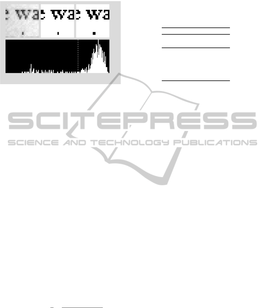
Figure 3: The upper left panel shows a noisy tile, whereas
the upper right panel shows the noise-free (ground truth)
tile. The upper middle panel shows the binarized version
of the noisy tile, using the optimal binarization threshold
indicated by a vertical dotted line in the histogram (lower
panel).
and the tile obtained by binarizing the noisy tile at the
current threshold, respectively. The sum extends over
all pixels in the image.
The procedure is illustrated in Figs. 3 and 4. The
top left panel of Fig. 3 shows a noisy tile (namely the
tile covering parts of the words he was in the docu-
ment image shown in Fig. 8 below) and the bottom
panel shows its (gray) histogram. The dotted line in
the histogram indicates the optimal threshold. The top
middle panel shows the image obtained by binarizing
the noisy tile with that threshold, and the top right
panel shows the corresponding clean tile. Fig 4 illus-
trates the process used for arriving at the best thresh-
old value: The figure shows the binarized tiles and
the PSNR values for a few different thresholds (T),
including the best threshold T
b
(178, in this case).
Now, the set H is supposed to contain represen-
tative histograms, together with their corresponding
optimal binarization thresholds, stored in the set T .
Thus, provided that the best threshold found (T
b
) ex-
ceeds a certain minimum (T
min
) as explained below,
the histogram of the current tile H is compared to all
the histograms (from other tiles) stored so far in the
set H = {H
0
, H
1
, . . .}, using the chi-square histogram
distance measure (Pele and Werman, 2010), defined
as
χ
2
(H
n
, H
m
) =
1
2
∑
k
(H
n
(k) − H
m
(k))
2
(H
n
(k) + H
m
(k))
, (3)
where H
q
(k) denotes the contents of bin k of his-
togram H
q
, q = n, m, and the sum extends over all
bins. If H is empty or the distance between the cur-
rent histogram H and histogram H
i
in H exceeds a
threshold d
tr
for all i, then H is added to H and the
threshold T
b
is added to the set of thresholds T . Thus,
Table 1: The seven parameters used in the binarizer. The
first two parameters, used during training, are described in
Subsect. 2.1 and the remaining five parameters, needed for
running the binarizer, are described in Subsect. 2.2.
Parameter Typical range
d
tr
[0.10, 0.20]
T
min
[5, 30]
d
use
[0.15, 0.25]
f [0.001, 0.01]
b [5, 30]
g [1.2, 3.0]
K [3, 10]
only histograms that are sufficiently different from the
ones already in H are stored.
The minimum allowed threshold T
min
is intro-
duced since, in cases where a tile has very low con-
trast and high brightness (i.e. such that most pixels are
very light gray), the training procedure may conclude,
based on the aggregate PSNR measure, that the opti-
mal binarization threshold should be very small (even
0), rendering the resulting binarized tile completely
white, thus (perhaps) losing some low-contrast text in
the process. Now, when running the binarizer (see be-
low) there is an option to enhance the contrast in the
tile, and this path should be taken if the contrast is
very low, i.e. if the tile either contains bright text on
a bright background (as in this example) or dark text
on a dark background (see Fig. 5). Thus, rather than
having the binarizer making a bright, low-contrast tile
completely white, the tile will instead be enhanced
(see below) so that, during the next pass, it can be
successfully binarized with a threshold T > T
min
(for
which a histogram might be available in H ). More-
over, in cases where no suitable matching histogram
can be found, even after repeated enhancement, the
resulting tile is made completely white in the final
step anyway, so again there is no need to store his-
tograms for which the associated threshold is very
small.
2.2 Using a Binarizer
Once the binarizer has been trained as described
above, and the five remaining parameters (described
below) in Table 1 have been set, it is ready for use.
The binarizer starts by dividing the image into tiles,
exactly as during training. Next, for each tile, the cor-
responding histogram H is computed. Then, the bina-
rizer runs through all the stored histograms H
i
in the
set H , computing the distance between H and H
i
, and
keeping track of the i that yields the smallest distance
(d
min
). If, after runningthrough all the histograms, the
smallest distance d
min
is smaller than the parameter
ICAART2014-InternationalConferenceonAgentsandArtificialIntelligence
36
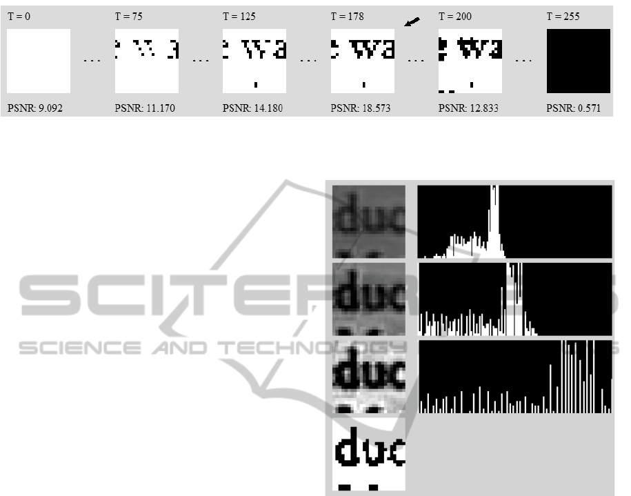
Figure 4: An illustration of the procedure used for finding the best binarization threshold for a single tile, namely the one
shown in Fig. 3. In this particular case, the best binarization threshold, indicated by an arrow in the figure, was found to be
178.
d
use
, the tile is binarized using the threshold T (from
the stored set T ) associated with the corresponding
histogram, i.e.
i = argmin dist(H, H
i
) (4)
and
T = T
i
(5)
If instead d
min
exceeds d
use
, the tile is enhanced, aim-
ing to increase the contrast so that a matching his-
togram can be found in the set H . The enhancement
procedure is similar to the one used in (Chen et al.,
2012). Here, the bin index i
f
(in the range [0, 255]),
containing a fraction f of the total number of pixels in
the image, is identified. Next, the (gray) pixel values
p
i, j
are enhanced as
p
i, j
← (p
i, j
− (i
f
+ b))g, (6)
where b is the brightness reduction factor and g is the
gain factor. If p
i, j
becomes negative, it is set to zero.
Likewise, if p
i, j
exceeds 255, it is set to 255.
In case enhancement is needed, the histogram
matching procedure describe above is then repeated
on the enhanced tile, either resulting in the tile be-
ing binarized (if a sufficiently close histogram match
is found) or another enhancement step being carried
out; see Fig. 5. In order to make sure that the algo-
rithm remains finite, a maximum of K iterations is al-
lowed. If no suitable binarization threshold has been
found even after K iterations, the corresponding tile is
set completely white. A flowchart showing the oper-
ation of the binarizer is provided in Fig. 6. Once all
tiles have been binarized, they are stitched together to
form a complete, binarized image.
Fig. 7 shows an example of the binarization of one
tile from one of the test images. Here, a sufficiently
close match was found, without enhancement. The
corresponding histogram (H
28
) is shown in the figure,
along with the binarized tile.
3 RESULTS
In order to test the method, a binarizer was trained, as
described in Subsect. 2.1 above, using a set of 10 arti-
Figure 5: An illustration of tile enhancement. In this case,
no matching histograms were found (in the set H of the
binarizer), neither for the original image shown in the top
panel along with its histogram, nor for the first enhanced
image, shown in the second panel from the top. How-
ever, after two enhancement steps, a matching histogram
was found for the histogram of the second enhanced tile,
shown in the third panel from the top. The binarized result
is shown in the bottom panel.
ficially generated training images, of the kind shown
in Fig. 1. Starting from a clean version of an image,
brightness variations and noise were added. Each im-
age was then divided into 16 × 10 tiles of 24 × 24
pixels each. Thus, during training, the binarizer en-
countered a total of 16× 10× 10 = 1600 histograms.
After some experimentation, the parameters T
min
and
d
tr
were set to 10 and 0.15, respectively. With the re-
quirements T
b
> T
min
and d
min
> d
tr
, a total of 102
histograms were kept during training. Note that the
number of histograms added typically decreases for
every additional training image. Thus, for example,
while 37 histograms were kept from the first train-
ing image, only one histogram was kept from the last
AMethodforDocumentImageBinarizationbasedonHistogram
MatchingandRepeatedContrastEnhancement
37
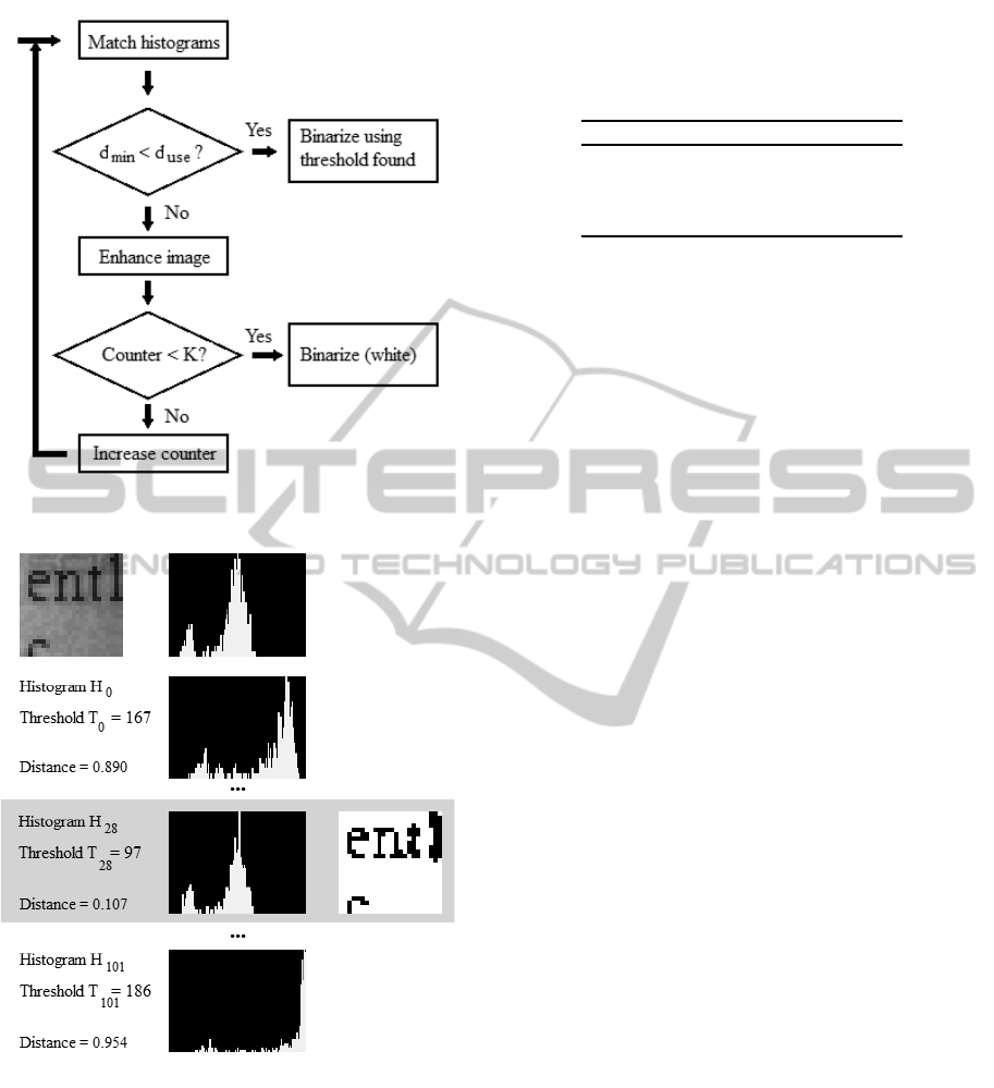
Figure 6: A flowchart showing the operation of the binarizer
during its use.
Figure 7: An example of tile binarization. The binarizer
generates the histogram (top panel) for the noisy tile, and
then runs through all the (102, in this case) histograms
stored during training, noting the histogram distances as de-
fined in Eq. 3. The best match, with a distance below the
minimum allowed distance (d
use
= 0.175, in this case), was
found for histogram 28, highlighted in gray. The resulting
binarized tile is shown as well.
training image: Before running through the last train-
ing image, the binarizer had already added 101 his-
tograms, covering most cases, so that only one ad-
ditional histogram was needed. A further discussion
of the accretive nature of the training method can be
Table 2: A comparison of the average binarization perfor-
mance, measured as the PSNR value obtained when com-
paring the binarized image generated from the binarizer to
the corresponding noise-free image.
Method Average PSNR
Otsu 6.457
Niblack 8.027
Sauvola 13.72
Proposed method 14.41
found in Sect. 4 below.
After completing the training, the binarizer was
applied to a set of five previously unseen test images.
The test images were also generated in pairs, so that
each pair contained a noisy version and a noise-free
(binarized) image. Of course, the binarizer was not
given information about the noise-free images during
testing: Those images were only use at the end, to
compute the performance measure; see Eq. 1. Even
though only five test images were used, they cov-
ered most of the possible variation in images of the
kind considered here, namely (web) camera images
of printed text documents such as, for example, let-
ters. Note also that the proposed method operates on
tiles, so that it is, effectively, applied several hundred
times (once per tile) to binarize the five test images.
Some earlier experimentation had given the fol-
lowing parameter values, which were used dur-
ing the test: d
use
= 0.175, f = 0.005, b = 20,
g = 2.2, and K = 3. Furthermore, the three
benchmark methods (Otsu’s method (Otsu, 1979),
Niblack’s method (Niblack, 1986), and Sauvola’s
method (Sauvola and Pietik¨ainen, 2000)) were also
applied to each of the five test images. It should be
noted that, for the type of images considered here,
i.e. (web) camera images of a printed document such
as a letter, Sauvola’s method in particular typically
does very well, and it therefore provides a challeng-
ing benchmark. The results are summarized in Ta-
ble 2. As can be seen, the proposed method outper-
formed the three other methods. The binarization re-
sults obtained for one of the test images is shown in
Fig. 8. For this particular image, the PSNR values
were 7.456 (Otsu), 8.498 (Niblack), 14.23 (Sauvola),
and 14.48 (proposed method). The proposed method
was also applied to some document images taken by
a web camera. An example is shown in Fig. 9, where
the upper panel shows the camera image and the lower
panel shows the result of applying the proposed bina-
rization method. Note that a standard preprocessing
step, which is not part of the binarizer, was applied to
sharpen the original camera image somewhat, result-
ing in the image shown in the upper panel of Fig. 9.
As can be seen, the resulting binarized image (lower
panel) is clearly readable, with the possible exception
ICAART2014-InternationalConferenceonAgentsandArtificialIntelligence
38
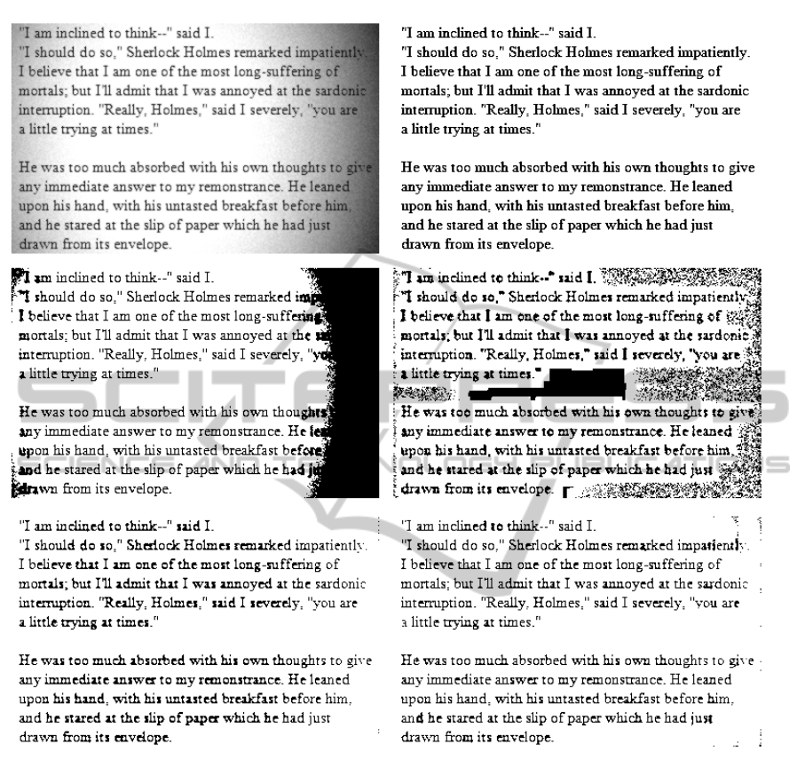
Figure 8: An example of the results obtained for one test image. The noisy version of the image is shown in the upper
left panel, whereas the upper right panel shows the clean, binarized version. In the middle row, the left panel shows the
binarization result obtained using Otsu’s method, and the right panel shows the result from applying Niblack’s method. In the
bottom row, the left panel shows the binarization results from Sauvola’s method (left panel) and the proposed method (right
panel).
of a few characters. This also indicates that the pro-
cedure for generating the artificial noisy images used
during training does result in images resembling real
camera images.
4 DISCUSSION AND
CONCLUSIONS
As can be seen above, the proposed method outper-
forms the benchmark methods. Moreover, it typically
achieves a rather constant line thickness of the text in
the binarized images. This can be seen in Fig. 8 by
comparing the proposed method (lower right panel)
to Sauvola’s method (lower left panel); for the latter,
the line thickness is more variable. For example, in
the right-most part of the image the text obtained with
Sauvola’s method is quite thin, whereas near the mid-
dle of the image, the characters are a bit too dark, so
that, for example, the holes in the characters a and
e are (incorrectly) filled; compare, for example, the
word admit in the two panels. On the other hand,
for this particular image, Sauvola’s method is slightly
better at eliminating noise in the right-most part of the
image. Nevertheless, the proposed method achieved
AMethodforDocumentImageBinarizationbasedonHistogram
MatchingandRepeatedContrastEnhancement
39
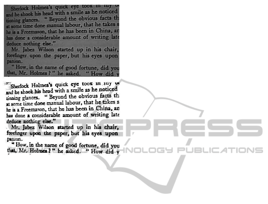
Figure 9: An example of the binarization results obtained
when applying the method to a document image obtained
from a web camera. Upper panel: The original image; lower
panel: The binarized image, obtained using the proposed
method.
a PSNR of 14.49, compared to 14.22 for Sauvola’s
method.
Since the binarizer contains a fairly large number
of histograms, one might be concerned about running
times. However, for the intended application, i.e. as
part of an intelligent agent able to read text in docu-
ment images, time is less of a concern than, say, for a
system that must operate in real-time with a rate of 10
or more frames per second. Of course, when reading
text in a document image out loud, the actual read-
ing takes many seconds, so that a small delay before
reading starts is not very important.
In any case, in its current configuration (which
has not been optimized for speed), the binarizer takes
around 0.36 ms per tile using a computer with an In-
tel Core i7-2600 CPU (3.40 GHz), meaning that the
training and test images used here take around 58 ms
to binarize, with a tile size of 24× 24 pixels. An im-
age of size 640 × 480 pixels would take around 195
ms to binarize. Note, however, that since the tiles are
processed independently of each other, there is ample
opportunity for a speed-up.
The main drawback with the proposed method, in
its current state at least, is that the user must specify
the number of tiles (or, rather, the tile size). The cor-
responding parameters (N and M) are not considered
to be part of the binarizer since, once a binarizer has
been trained, it should work well with other tile sizes
also, at least within a certain range. The tiles must
be able to generate a reasonably accurate histogram,
implying that they cannot be made too small; at least
a few hundred pixels are needed. On the other hand,
the tiles must be small enough so that the brightness
does not vary too much over a tile. However, even
with some brightness variation, a tile can normally be
binarized successfully, making it quite easy to set a
suitable tile size for a given class of images (say, let-
ters with standard font size, held at a distance of 0.5 m
from a camera). In fact, the tile size used here (24×24
pixels) typically works very well, except in extreme
cases (e.g. images with huge characters, of a kind not
usually found in letters).
Still, in future work, an effort will be made to au-
tomatize the tile size selection. This can be done by
starting with large tiles, and then further subdividing
those tiles for which the estimated brightness varia-
tion is above a certain threshold. In addition, rather
than setting the seven parameters manually, one may
consider applying some form of optimization algo-
rithm, e.g. particle swarm optimization (Kennedy and
Eberhart, 1995). However, one should note that the
parameter ranges are quite narrow (see Table 1) so
that the values can generally be set by hand.
One can also note that the training method can be
used accretively, i.e. if, at some point, it is deemed
that the binarizer’s performance is inadequate, per-
haps because it is lacking some crucial histograms
due to insufficient training, one can then add his-
tograms by simply extending the training method over
a few more training images, without having to start
from an empty set of histograms. This implies that
if one happens to end the training procedure prema-
turely, so that the binarizer does not contain a suffi-
cient number of histograms for reliable binarization,
the problem can easily be rectified.
Regarding training, it can be carried out very
quickly with a training set of the kind used here,
i.e. one that consists of pairs of artificially generated
images, one noisy and one clean, such that the latter
can be used as a ground truth. On the other hand, in
order to obtain the best performance possible over ac-
tual camera images (which might also be bent, stained
etc.), it would probably be better to train the bina-
rizer using such images, the problem being that in
such a case one would not, of course, have an exact,
ground truth image (at least not without considerable
effort) to compare with. However, one could use a
subjective method for binarizing the tiles of the train-
ing images, focusing on perceived readability of the
letters. It should also be noted that the PSNR mea-
ICAART2014-InternationalConferenceonAgentsandArtificialIntelligence
40

sure is an aggregate measure for the whole tile, and
therefore sometimes the human eye can be better than
the PSNR measure at judging the optimal binarization
threshold. Thus, one could attempt a semi-automatic
method, where the computer program keeps track of
histogram distances and also presents tiles, one at a
time, to a human user, along with all the 256 possible
binarizations of the tile in question, letting the human
user decide on the optimal threshold. The training
will then be more time-consuming, but can be carried
out once and for all, and might give even better bina-
rization results. The development of such a procedure
is currently underway. To conclude, one can note that
the proposed method is able to binarize document im-
ages with noise and brightness variations, achieving
better performance than several benchmark methods.
ACKNOWLEDGEMENTS
The author gratefully acknowledges financial support
from De blindas v
¨
anner.
REFERENCES
Chen, K.-N., Chen, C.-H., and Chang, C.-C. (2012). Ef-
ficient illumination compensation techniques for text
images. Digital Signal Processing, 22:726–733.
Gonz´alez, A. and Bergasa, L. (2013). A text reading algo-
rithm for natural images. Image and vision computing,
31:255–274.
Kennedy, J. and Eberhart, R. C. (1995). Particle swarm op-
timization. In Proceedings of the IEEE International
Conference on Neural Networks, pages 1942–1948.
Lu, S., Su, B., and Tan, C. (2010). Document image
binarization using background estimation and stroke
edges. International Journal on Document Analysis
and Recogntion, 13(4):303–314.
Neumann, L. and Matas, J. (2010). A method for text local-
ization and recognition in real-world images. In 10th
Asian Conference on Computer Vision (ACCV2010),
LNCS 6495, pages 2067–2078.
Niblack, W. (1986). An Introduction to Image Processing.
Prentice-Hall.
Otsu, N. (1979). A threshold selection method from gray-
level histograms. IEEE Transactions on Systems,
Man, and Cybernetics, 9:62–66.
Pele, O. and Werman, M. (2010). The quadratic-chi his-
togram distance family. In 11th European Conference
on Computer Vision (ECCV2010), LNCS 6312, pages
749–762.
Sauvola, J. and Pietik¨ainen, M. (2000). Adaptive document
image binarization. Pattern Recognition, 33:225–236.
Shi, J., Ray, N., and Zhang, H. (2012). Shape based lo-
cal thresholding for binarization of document images.
Pattern Recognition Letters, 33:24–32.
Stathis, P., Kavallieratou, E., and Papamarkos, N.
(2008). An evaluation technique for binarization al-
gorithms. Journal of Universal Computer Science,
14(18):3011–3030.
Valizadeh, M. and Kabir, E. (2013). An adaptive water
flow model for binarization of degraded document im-
ages. International Journal on Document Analysis
and Recogntion, 16(2):165–176.
AMethodforDocumentImageBinarizationbasedonHistogram
MatchingandRepeatedContrastEnhancement
41
