Improving Color Constancy in the Presence of Multiple Illuminants

using Depth Information

Marc Ebner and Johannes Hansen

Ernst-Moritz-Arndt-Universit

at Greifswald, Institut f

ur Mathematik und Informatik,

Walther-Rathenau-Straße 47, 17487 Greifswald, Germany

Keywords:

Color Constancy, Space Average Color, Depth Map, Color, Kinect.

Abstract:

A human observer is able to judge the color of objects independent of the illuminant. In contrast, a digital sen-

sor (or the retinal receptors for that matter) only measure reﬂected light which varies with the illuminant. The

brain is somehow able to compute a color constant descriptor from the light falling onto the retina. We have

improved a well known color constancy algorithm based on local space average color. This color constancy

algorithm can be mapped to the different visual processing stages of the human brain. We have extended this

algorithm by incorporating depth information. The idea is that wherever there are depth discontinuities there

may also be a change of the illuminant in the image. Hence, depth discontinuities are used to separate differ-

ent illuminants. This allows us to better estimate the local illumination and allows us to compute an improved

color constant descriptor. We also compute local space average depth to decide locally whether to average data

from retinal sensors uniformly or non-uniformly. We show how our algorithm works on real world scenes.

Depth information is obtained from a standard Kinect sensor.

1 INTRODUCTION

Object color is an important cue in everyday life. We

use it to recognize or distinguish different objects.

However, color is a product of the brain (Zeki, 1993).

The brain somehow computes a color constant de-

scriptor from the data measured by the retinal recep-

tors (Ebner, 2007a). The ability to compute a color

constant descriptor is also very important for artiﬁ-

cial vision systems. In particular, it is very important

in the area of autonomous mobile robotics whenever

robots have to work in several different environments.

In the human eye, the retinal receptors measure

light reﬂected by objects. Unfortunately, reﬂected

light varies with the spectral power distribution of

the illuminant. Suppose a white wall is illuminated

by an illuminant with a power distribution having a

maximum in the red part of the spectrum. Hence

the cones with a maximum absorption in the red part

of the spectrum will respond more strongly than the

cones with maximum absorption in the green and blue

parts of the spectrum. Similarly, if we take a digital

camera and take a digital photo of this scene, then

the image will have a strong reddish color cast to it.

The wall will appear red in the image. If the illu-

minant is known, we can compute a color corrected

image of the scene. The scene will then look as if it

had been illuminated by a uniform illuminant. Dig-

ital cameras assume that a single uniform illuminant

(sunlight, cloudy sky, ﬂash, neon light, etc.) is illu-

minating the scene. Hence, a digital camera corrects

for a single illuminant. However, in practice this as-

sumption (that a single illuminant is illuminating the

scene) is not valid. We usually have multiple different

illuminants such as sunlight falling through a window

and artiﬁcial light turned on inside the building. Thus,

we need to estimate the illuminant locally in order to

correctly estimate object reﬂectance, i.e. the percent-

age of incident light which is reﬂected by an object.

This estimate of object reﬂectance can then be used

for object recognition as it is independent of the illu-

minant.

A number of different color constancy algorithms

have been proposed (Agarwal et al., 2006; Ebner,

2007a). Most algorithms assume that a single uniform

illuminant is illuminating the scene, e.g. the White

Patch Retinex algorithm or the gray world assumption

(Buchsbaum, 1980). Some algorithms assume that

the illuminant is somehow constrained (Finlayson and

Hordley, 2001). A color constancy algorithm based

on the gray-edge hypothesis has been proposed by

van de Weijer et al. (2007). Apart from the original

133

Ebner M. and Hansen J..

Improving Color Constancy in the Presence of Multiple Illuminants using Depth Information.

DOI: 10.5220/0004743601330140

In Proceedings of the International Conference on Bio-inspired Systems and Signal Processing (BIOSIGNALS-2014), pages 133-140

ISBN: 978-989-758-011-6

 2014 SCITEPRESS (Science and Technology Publications, Lda.)

Retinex algorithm (Land and McCann, 1971), only a

few work in the context of non-uniform illumination,

e.g. Barnard et al.’s (1997) extension of the gamut

constraint algorithm. In practice, one usually has to

cope with a non-uniform illumination.

Most algorithms for color constancy cannot be

readily mapped to the human vision system. Ebner

(2007c; 2012) has proposed a model of human color

perception which can be mapped to the human vision

system. His method also works in the context of non-

uniform illumination. In its original form, this algo-

rithm only uses the output from the retinal receptors

to arrive at a color constant descriptor. It does not use

depth information. This algorithm has been extended

by Ebner and Hansen (2013) to incorporate depth in-

formation. Here, we also compute local space average

depth in order to decide locally whether to average

data from retinal senors uniformly or non-uniformly.

In addition, we better handle uncertainty in the posi-

tion of the detected edges.

Depth information is readily available inside the

human vision system. Gilchrist (1977) has put for-

ward the coplanar ratio hypothesis. According to this

hypothesis, lightness is determined primarily by ratios

within perceived planes. Our research is in line with

this hypothesis. How and if depth cues are actually

used by the human visual system to compute a color

constant descriptor is currently unknown. With this

contribution we explore how depth information may

be used to arrive at a color constant descriptor. For ar-

tiﬁcial vision systems, we can obtain depth informa-

tion from a variety of methods (Horn, 1986; Jain et al.,

1995). For our experiments, we have used the Kinect

sensor to obtain a RGB image and the so called depth

map which provides the distance to the corresponding

object point for each pixel of the image.

In Section 2 we brieﬂy explain Ebner’s algorithm

and how it can be mapped to the individual stages of

the human vision system. In Section 3 we explain

how depth information can be integrated into this al-

gorithm. Section 4 describes how we have used the

Kinect sensor to obtain a dense depth map. Section

5 describes the experiments that we have performed.

Section 6 concludes this paper.

2 COLOR CONSTANCY BASED

ON LOCAL SPACE AVERAGE

COLOR

A color constant descriptor can be computed in var-

ious different ways. See Ebner (2007a) or Barnard

et al. (2002) for an overview and evaluation of sev-

eral different algorithms. A quite simple algorithm is

the gray world assumption which has been put for-

ward by Buchsbaum (1980). According to the gray

world assumption, the world is gray on average. This

assumption allows us to compute a color constant de-

scriptor. Using this assumption, we can obtain an es-

timate of the illuminant by simply averaging all pixel

values. Given this estimate, we can compute an out-

put image that is independent of the illuminant. For

the gray world assumption to work, it is necessary that

quite a large number of different surface reﬂectances

are contained in the scene being viewed.

Ebner (2009) has extended this algorithm to esti-

mate the illuminant locally for each image pixel. He

has also shown how this algorithm can be mapped to

the human vision system (Ebner, 2007c, 2012). The

algorithm runs on a grid of processing elements. It

is assumed that we have one processing element per

image pixel. For each pixel, we have three color

bands in the red, green and blue parts of the spec-

trum. The processing elements are laterally con-

nected to each other. Each processing element es-

timates the illuminant for the corresponding image

pixel by computing local space average color. Let

a(x,y) = [a

(x,y),a

(x,y)] be local space av-

erage color estimated by processing element at posi-

tion (x, y). Let c(x,y) = [c

(x,y),c

(x,y)] be

the measured color, i.e. the pixel color of the input

image, at position (x,y). It is assumed that c(x,y) cor-

responds linearly to the irradiance falling onto the im-

age sensor. Let N(x,y) be the neighborhood deﬁned

for the processing element at position (x,y) and let p

be a small positive value. The following two update

equations are iterated until convergence:

(x,y) =

|N(x,y)|

∑

)∈N(x,y)

) (1)

(x,y) =(1 − p

(x,y) + p

(x,y) (2)

with i ∈ {r,g,b}. The ﬁrst equation takes local space

average color from neighboring processing elements

and averages it. The current element can also be in-

cluded in this averaging process. The second equation

adds a tiny amount of the measured color to the esti-

mated average.

The parameter p

determines the extent of the av-

eraging. If p

is rather small, then local space aver-

age color is computed over an extensive area. If p

is comparatively large, then local space average color

is computed over a very small area. The parameter

is usually set such that a sufﬁciently large number

of image pixels are included in the average, e.g. 30%

of all image pixels. Let ¯p

be the desired percentage

of the image over which local space average color is

computed and let s be the maximum of the width and

BIOSIGNALS2014-InternationalConferenceonBio-inspiredSystemsandSignalProcessing

134

the height of the image in pixels, then p

is given by

= 1/(4 ∗ ¯p

Assuming narrow band sensors, then the mea-

sured irradiance is proportional to the reﬂectance

(x,y) and irradiance L

(x,y) at the images object

point for color band or wavelength i. In other words,

we have c

(x,y) = L

(x,y)R

(x,y) assuming a scaling

factor of 1. Using L

(x,y) ∝ a

(x,y) we can compute

a color constant descriptor by dividing the measured

color c

(x,y) by local space average color a

(x,y).

In Ebner’s (2012) model, the retinal receptors

measure the irradiance falling into the eye. The reti-

nal receptors have a logarithmic response curve. The

color space is rotated due to color opponent cells be-

fore reaching the visual cortex. Cells in V4 compute

local space average color. This local space average

color is subtracted from the data made available by

cells in V1. Because of the logarithmic response, lo-

cal space average color simply needs to be subtracted

from the data from V1 in order to arrive at a color

constant descriptor.

Within area V1, the visual stimulus is analyzed

with respect to all kinds of different aspects (Living-

stone and Hubel, 1984). Cells have been found whose

optimal stimulus is an oriented line. Other cells’ opti-

mal stimulus is light of a particular wavelength. Cells

usually respond more prominently to one eye or the

other. These cells are grouped in columns which are

called ocular dominance columns. It could be that vi-

sual information is also analyzed with respect to depth

discontinuities in order to improve color perception.

We will explore this possibility in the next section.

3 USING DEPTH INFORMATION

TO IMPROVE COLOR

CONSTANCY

In a natural scene, there are usually many different

illuminants. Sun light may be falling through a win-

dow, a desk lamp may be turned on and at the same

time neon light may illuminate the interior of the

room. If we take an image of the room, the top of the

desk may be illuminated by the light from the desk

lamp while the area below the desk may be illumi-

nated by ambient light which has been reﬂected mul-

tiple times by the objects contained in the room. If we

look at the desk, we see a depth discontinuity at the

edge of the desk which separates the top of the desk

from the ﬂoor.

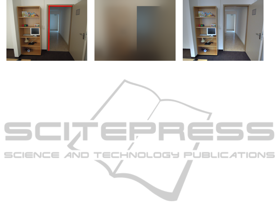
Figure 1(a) shows another example. The ﬁrst

room is illuminated by sunlight falling through a win-

dow while the corridor is illuminated by a blueish illu-

minant. For this image, the door frame provides a nice

separation between the two illuminants. The depth

discontinuity at the door frame has been highlighted

manually.

We will now show how we can integrate such

depth discontinuities into the algorithm to compute

local space average color. It does not make sense to

average local space average color across depth dis-

continuities because it is assumed that one illuminant

illuminates the area on one side of the edge while an-

other illuminant illuminates the area on the other side

of the edge. Figure 1(b) shows an estimate of the two

illuminants (computed by our algorithm). The two

illuminants are clearly separated by the door frame.

On the right hand side of the door we have a smooth

illumination gradient. Figure 1(c) shows the output

image which has been computed by dividing the mea-

sured color c(x,y) shown in Figure 1(a) by local space

average color a(x, y) shown in Figure 1(b).

Of course it is also possible that the same illumi-

nant illuminates both sides of an edge. However, this

will do no harm. In order to take depth discontinuities

into account, we only need to use a slightly modiﬁed

neighborhood N

(x,y) which replaces the uniform

neighborhood N(x, y) in Equation (1). Let d(x,y) be

the depth map. The depth map speciﬁes the distance

from the camera to each object point. We only want

to average across processing elements whose corre-

sponding object points have approximately the same

depth. Hence, we can deﬁne N

(x,y) as follows

(x,y) ={(x

) ∈ N(x,y)

with |d(x,y) −d(x

)| ≤ ε

(x,y)}

(3)

where ε

deﬁnes the edge threshold assuming that the

depth map has been scaled to the range [0, 1]. We av-

erage across discontinuities smaller than ε

(x,y). Dis-

continuities larger than ε

(x,y) separate two process-

ing elements in the averaging process.

The threshold ε

can be set to a ﬁxed value for

the entire image. However, using a locally varying

threshold may be more appropriate. Hence, we also

compute local space average depth. Local space av-

erage depth

d is computed using the same method we

have used to compute local space average color

(x,y) =

|N(x,y)|

∑

)∈N(x,y)

) (4)

d(x,y) =(1 − p

)

(x,y) + p

d(x,y) (5)

where d(x,y) is the depth value at position (x,y) and

is a small value which determines the extent of

the averaging of the depth map. The parameter ¯p

is deﬁned in exactly the same way as the parameter

¯p

above. Now that we have computed local space

ImprovingColorConstancyinthePresenceofMultipleIlluminantsusingDepthInformation

135

(a) (b) (c)

Figure 1: (a) Sample image with two illuminants. The depth discontinuity separating the two illuminants has been manually

highlighted in red. (b) Estimate of the illuminant. (c) Color constant descriptor.

average depth, we can make the threshold dependent

on local depth. E.g. ε

(x,y) = 0.1

d(x,y) means that

we do not average across depth differences larger than

10% of the average depth in the region.

In practice, the alignment between the depth map

and the color map may not be perfect. A non-perfect

alignment between the depth map and the color im-

age may result in artefacts at regions where the il-

luminant from another nearby region is used instead

of the correct illuminant. That’s why we ﬁrst com-

pute depth edges. A depth edge is located between

two neighboring points (x,y) and (x

) if we have

|d(x,y) −d(x

)| > ε

(x,y). We dilate the resulting

binary edge image using a square structuring element

of size 5 ×5. The size of the structuring element is

set to the size of the uncertainty in the alignment be-

tween the depth map and the color image. The depth

discontinuity is then assumed to be located inside this

enlarged area at a location where we also have a color

edge with a threshold of ε

= 0.1. Because of this op-

eration, depth discontinuities are now in perfect align-

ment with color edges in the image. If we have the un-

likely case of a depth edge between two pixels but no

color edge then our method will average across these

pixels. In the human visual system, it is known that

different aspects such as color, shape and motion are

processed by different visual areas (Zeki, 1993; Zeki

et al., 1991). It may be that these aspects are brought

into alignment by a dynamic process similar to the

one shown by Ramachandran (1993).

Figure 2 compares the two threshold methods for

a real scene. Figure 2(a) shows the input image. Fig-

ure 2(b) shows local space average color computed

with a ﬁxed threshold for the entire image while Fig-

ure 2(c) shows local space average color computed

with a spatially varying threshold as described above.

The delineation of the border between the different

illuminants is more accurate with a spatially varying

threshold.

In the human vision system, binocular disparity

can be used to estimate the distance of object points

relative to the observer. For our experiments, we have

used the Kinect to obtain a depth map for each input

image.

4 OBTAINING A KINECT IMAGE

ALIGNED DEPTH MAP

The Kinect sensor has been developed by Microsoft

for the Xbox 360 video game console (Microsoft Cor-

poration, 2011). It is a sensor which can be used for

motion tracking and also sound position tracking. It

consists of a horizontal bar with a RGB camera, a

depth sensor, a multi-array microphone which rests on

a motorized tilt unit as shown in Figure 3(a). Figure

3(b) shows the RGB image obtained with the Kinect

sensor for a sample scene. The corresponding depth

map is shown in Figure 3(c). A detailed description of

the Kinect sensor is given by Koﬂer (2011). To date, it

has been used in numerous different research projects.

For instance, Newcombe et al. (2011), have shown

how to perform dense surface mapping and tracking

with the Kinect sensor. Gabel et al. (2012) have used

it for full body gait analysis. A detailed evaluation of

the Kinect sensor for computer vision applications is

given by Andersen et al. (2012).

In order to use this depth map, we need to estab-

lish a correspondence between each image pixel of the

input image and each pixel of the depth map. Color

and depth sensors are a small distance apart from each

other and they do not necessarily point into the same

direction. The intrinsics and extrinsics of the sensors

differ. The depth sensor covers a signiﬁcantly smaller

area than the color sensor. In addition, the depth sen-

sor outputs data with a non-linear correspondence to

distance.

We align the RGB input image and the depth map

by performing a stereo calibration, i.e. computing

intrinsic and extrinsic parameters of the two cam-

eras and then transform the depth value to distance

BIOSIGNALS2014-InternationalConferenceonBio-inspiredSystemsandSignalProcessing

136

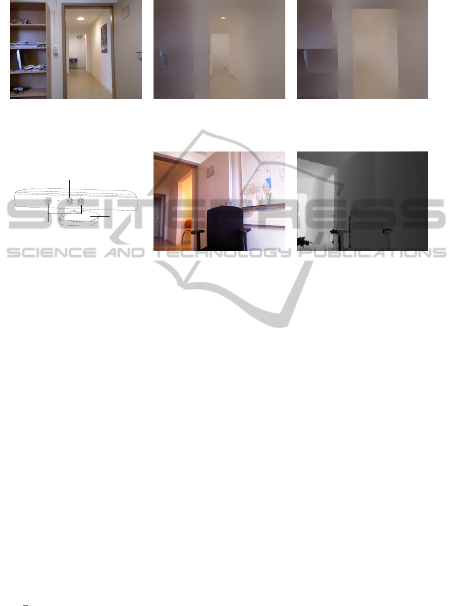
(a) (b) (c)

Figure 2: (a) Input image. (b) local space average color with a ﬁxed threshold ε

(x,y) = ε

. (c) local space average color with

a spatially varying threshold ε

(x,y) = 0.1

d(x, y). In addition, depth discontinuities are aligned with color edges.

XBOX 360

RGB Camera

Depth Sensor

Tilt Unit

(a) (b) (c)

Figure 3: (a) Kinect sensor. (b) RGB image (c) Depth map.

in meters. This approach is also described by Burrus

(http://openkinect.org) and Koﬂer (2011). The Kinect

sensor is not able to compute depth information for all

pixels due to occlusion. Due to the arrangement of the

infrared camera and the infrared laser which produces

the laser grid for depth computation, the grid may not

be visible for certain areas seen by the camera. This

always happens to the left side of an edge. In order

to accurately detect such edges, we need to compute a

dense depth map from the Kinect output. We do this

by iteratively ﬁlling in data from the left hand side.

We call pixels for which the Kinect was able to esti-

mate a depth value “a valid depth value” and we call

all other pixels “invalid depth values”. Before we ap-

ply our algorithm, we ﬁlter the depth map by remov-

ing isolated valid depth values which are surrounded

by invalid depth values. These depth values are as-

sumed to be incorrect. We then iterate n

times over

the image. Within each row with invalid pixels, we

start from the left hand side and loop over all pixels

with invalid depth values from left to right. Each pixel

with an invalid depth value is updated by interpolat-

ing depth values from the top, upper left, left, lower

left and the bottom side. The values from the top, left

and bottom side use a weight of 1 while the diagonal

pixels from the upper left and lower left use a weight

of 1/

√

2. We end up with a dense depth map which

we can use for our algorithm.

5 EXPERIMENTS AND RESULTS

The algorithm is tested on a number of different im-

ages. Unfortunately, the Kinect only offers a rela-

tively small ﬁeld of view. The depth sensor provides

data in the range from 0.8 to 3.5 meters with a depth

resolution of 1cm at a distance of 2m (Andersen et al.,

2012). This constrains the types of scenes that we can

shoot. We have taken care to avoid shiny surfaces,

such as mirrors, polished metals or brilliant varnishes

in the scene. Such surfaces irritate the depth sensor.

For dark scenes, noise can be removed by taking mul-

tiple images and then averaging the output.

The Kinect computes a depth map of size 640 ×

480. The alignment algorithm corrects for the dif-

ferences between the RGB image and the depth map.

Since the RGB image and the depth map are not per-

fectly registered, we obtain a border around the im-

age where depth is undeﬁned. Hence, we crop the

images to size 569 ×428 for further processing. The

parameters were set to ¯p

= 0.25, ¯p

= 0.1, ε

(x,y) =

0.1

d(x,y), n

= 15 and ε

= 0.1.

Figure 4 shows the results. For comparison Fig-

ure 5 through Figure 8 shows the estimate of the il-

luminant, i.e. local space average color for images 1

through 4, computed with three other color constancy

algorithms: the gray world assumption (GW), stan-

dard local space average color (LSA) (Ebner, 2009),

ImprovingColorConstancyinthePresenceofMultipleIlluminantsusingDepthInformation

137

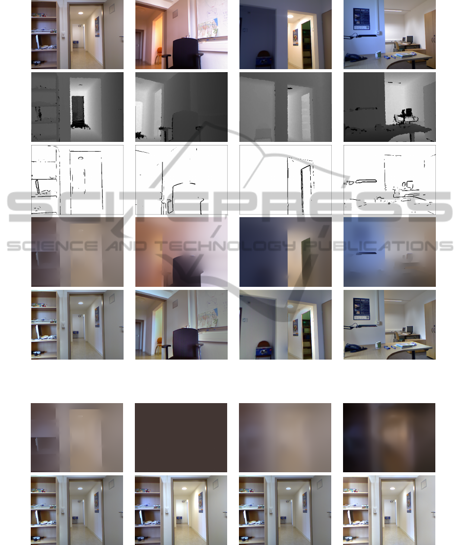
1 2 3 4

input imagedepth mapedges

ill. estimate

output

Figure 4: Results of our algorithm for 4 sample images.

Depth Map-LSA GW LSA Iso-LSA

ill. estimate

output

Figure 5: Comparison with three other color constancy algorithms for image 1: gray world assumption (GW), local space

average color (LSA), computation of anisotropic local space average color along iso-illumination lines (Iso-LSA).

and computation of anisotropic local space average

color along iso-illumination lines (Iso-LSA) (Ebner,

2007b). None of these methods use depth informa-

tion. When we compare the results we see that depth

information allows us to obtain a better estimate of

the illuminant in the vicinity of depth edges.

BIOSIGNALS2014-InternationalConferenceonBio-inspiredSystemsandSignalProcessing

138

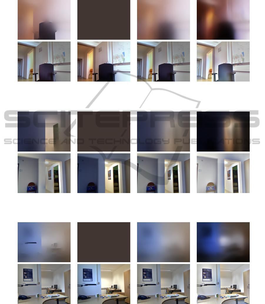
Depth Map-LSA GW LSA Iso-LSA

ill. estimate

output

Figure 6: Comparison with three other color constancy algorithms for image 2: gray world assumption (GW), local space

average color (LSA), computation of anisotropic local space average color along iso-illumination lines (Iso-LSA).

Depth Map-LSA GW LSA Iso-LSA

ill. estimate

output

Figure 7: Comparison with three other color constancy algorithms for image 3: gray world assumption (GW), local space

average color (LSA), computation of anisotropic local space average color along iso-illumination lines (Iso-LSA).

Depth Map-LSA GW LSA Iso-LSA

ill. estimate

output

Figure 8: Comparison with three other color constancy algorithms for image 4: gray world assumption (GW), local space

average color (LSA), computation of anisotropic local space average color along iso-illumination lines (Iso-LSA).

6 CONCLUSIONS

We have shown how depth information can help in

improving illumination estimates. A well known al-

gorithm for color constancy based on local space av-

erage color has been updated to also include depth

information. For our experiments, we have used the

Kinect sensor to provide an RGB image with a cor-

ImprovingColorConstancyinthePresenceofMultipleIlluminantsusingDepthInformation

139

responding depth map. Depth discontinuities in the

depth map are assumed to separate different illumi-

nants from each other. Our algorithm was tested on

several different sample images. Comparison results

with three other color constancy algorithms are also

shown.

REFERENCES

Agarwal, V., Abidi, B. R., Koschan, A., and Abidi, M. A.

(2006). An overview of color constancy algorithms.

Journal of Pattern Recognition Research, 1(1):42–54.

Andersen, M. R., Jensen, T., Lisouski, P., Mortensen, A. K.,

Hansen, M. K., Gregersen, T., and Ahrendt, P. (2012).

Kinect depth sensor evaluation for computer vision

applications. Technical Report ECE-TR-6, Aarhus

University, Denmark.

Barnard, K., Cardei, V., and Funt, B. (2002). A comparison

of computational color constancy algorithms – part I

and II. IEEE Trans. on Image Processing, 11(9):972–

996.

Barnard, K., Finlayson, G., and Funt, B. (1997). Color con-

stancy for scenes with varying illumination. Computer

Vision and Image Understanding, 65(2):311–321.

Buchsbaum, G. (1980). A spatial processor model for object

colour perception. Journal of the Franklin Institute,

310(1):337–350.

Ebner, M. (2007a). Color Constancy. John Wiley & Sons,

England.

Ebner, M. (2007b). Estimating the color of the illumi-

nant using anisotropic diffusion. In Kropatsch, W. G.,

Kampel, M., and Hanbury, A., eds., Proc. of the 12th

Int. Conf. on Computer Analysis of Images and Pat-

terns, Vienna, Austria, pp. 441–449, Berlin. Springer-

Verlag.

Ebner, M. (2007c). How does the brain arrive at a color con-

stant descriptor? In Mele, F., Ramella, G., Santillo, S.,

and Ventriglia, F., eds., Proc. of the 2nd Int. Symp. on

Brain, Vision and Artiﬁcial Intelligence, Naples, Italy,

pp. 84–93, Berlin. Springer.

Ebner, M. (2009). Color constancy based on local space av-

erage color. Machine Vision and Applications Journal,

20(5):283–301.

Ebner, M. (2012). A computational model for color per-

ception. Bio-Algorithms and Med-Systems, 8(4):387–

415.

Ebner, M. and Hansen, J. (2013). Depth map color con-

stancy. Bio-Algorithms and Med-Systems (accepted).

Finlayson, G. and Hordley, S. (2001). Colour signal pro-

cessing which removes illuminant colour temperature

dependency. UK Patent Application GB 2360660A.

Gabel, M., Gilad-Bachrach, R., Renshaw, E., and Schuster,

A. (2012). Full body gait analysis with Kinect. In

Proc. of the Annual Int. Conf. of the IEEE Engineering

in Medicine and Biology Society, San Diego, CA, pp.

1964–1967. IEEE.

Gilchrist, A. L. (1977). Perceived lightness depends on per-

ceived spatial arrangement. Science, 195:185–187.

Horn, B. K. P. (1986). Robot Vision. The MIT Press, Cam-

bridge, MA.

Jain, R., Kasturi, R., and Schunck, B. G. (1995). Machine

Vision. McGraw-Hill, Inc., New York.

Koﬂer, M. (2011). Inbetriebahme und untersuchung des

Kinect sensors. Master’s thesis, FH Ober

osterreich,

Osterreich.

Land, E. H. and McCann, J. J. (1971). Lightness and retinex

theory. Journal of the Optical Society of America,

61(1):1–11.

Livingstone, M. S. and Hubel, D. H. (1984). Anatomy and

physiology of a color system in the primate visual cor-

tex. The Journal of Neuroscience, 4(1):309–356.

Microsoft Corporation (2011). Programming with the

Kinect for Windows SDK.

Newcombe, R. A., Izadi, S., Hilliges, O., Molyneaux, D.,

Kim, D., Davison, A. J., Kohli, P., Shotton, J., Hodges,

S., and Fitzgibbon, A. (2011). Kinectfusion: Real-

time dense surface mapping and tracking. In Proc. of

the 10th IEEE Int. Symp. on Mixed and Augmented

Reality, pp. 127–136. IEEE.

Ramachandran, V. S. (1993). Filling in gaps in perception:

Part II. Scotomas and phantom limbs. Current Direc-

tions in Psychological Science, 2(2):56–65.

van de Weijer, J., Gevers, T., and Gijsenij, A. (2007). Edge-

based color constancy. IEEE Trans. on Image Pro-

cessing, 16(9):2207–2214.

Zeki, S. (1993). A Vision of the Brain. Blackwell Science,

Oxford.

Zeki, S., Watson, J. D. G., Lueck, C. J., Friston, K. J.,

Kennard, C., and Frackowiak, R. S. J. (1991). A

direct demonstration of functional specialization in

human visual cortex. The Journal of Neuroscience,

11(3):641–649.

BIOSIGNALS2014-InternationalConferenceonBio-inspiredSystemsandSignalProcessing

140