
Precise 3D Pose Estimation of Human Faces
´
Akos Pernek
1,2
and Levente Hajder
1
1
Computer and Automation Research Institute, Hungarian Academy of Sciences, Kende u. 13-17, 1111-Budapest, Hungary
2
Department of Automation and Applied Informatics, Budapest University of Technology and Economics,
M
˝
uegyetem rakpart 3-9, 1111-Budapest, Hungary
Keywords:
Structure from Motion, Symmetric Reconstruction, Non-rigid Reconstruction, Facial Element Detection, Eye
Corner Detection.
Abstract:
Robust human face recognition is one of the most important open tasks in computer vision. This study deals
with a challenging subproblem of face recognition: the aim of the paper is to give a precise estimation for the
3D head pose. The main contribution of this study is a novel non-rigid Structure from Motion (SfM) algorithm
which utilizes the fact that the human face is quasi-symmetric. The input of the proposed algorithm is a set of
tracked feature points of the face. In order to increase the precision of the head pose estimation, we improved
one of the best eye corner detectors and fused the results with the input set of feature points. The proposed
methods were evaluated on real and synthetic face sequences. The real sequences were captured using regular
(low-cost) web-cams.
1 INTRODUCTION
The shape and appearance modeling of the human
face and the fitting of these models have raised signif-
icant attention in the computer vision community. Till
the last few years, the state-of-the-art method used
for facial feature alignment and tracking was the ac-
tive appearance model (AAM) (Cootes et al., 1998;
Matthews and Baker, 2004). The AAM builds a sta-
tistical shape (Cootes et al., 1992) and grey-level ap-
pearance model from a face database and synthesizes
the complete face. Its shape and appearance param-
eters are refined based on the intensity differences of
the synthesized face and the real image.
Recently, a new model class has been developed
called the constrained local model (CLM) (Cristi-
nacce and Cootes, 2006; Wang et al., 2008; Saragih
et al., 2009). The CLM model is in several ways
similar to the AAM, however, it learns the appear-
ance variations of rectangular regions surrounding the
points of the facial feature set.
Due to its promising performance, we utilize the
CLM for facial feature tracking. Our C++ CLM im-
plementation is mainly based on the paper (Saragih
et al., 2009), however, it utilizes a 3D shape model.
The CLM (so as the AAM) requires a training
data set to learn the shape and appearance variations.
We use a basel face model (BFM) (P. Paysan and
R. Knothe and B. Amberg and S. Romdhani and T.
Vetter, 2009)-based face database for training data
set. The BFM is a generative 3D shape and texture
model which also provides the ground-truth head pose
and the ground-truth 2D and 3D facial feature coor-
dinates. Our training database consists of 10k syn-
thetic faces of random shape and appearance. The 3D
shape model or the so-called point distribution model
(PDM) of the CLM were calculated from the 3D fa-
cial features according to (Cootes et al., 1992).
During our experiments we have identified that the
BFM-based 3D CLM produces low performance at
large head poses (above 30 degree). The CLM fit-
ting in the eye regions showed instability. We pro-
pose here two novelties: (i) Since the precision of eye
corner points are of high importance for many vision
applications, we decided to replace the eye corner es-
timates of the CLM with that of our eye corner detec-
tor. (ii) We propose a novel non-rigid structure from
motion (SfM) algorithm which utilize the fact that hu-
man face is quasi-symmetric (almost symmetric).
2 EYE CORNER DETECTION
One contribution of our paper is a 3D eye corner de-
tector inspired by (Santos and Proenc¸a, 2011). The
main idea of our method is that the 3D information
increases the precision of eye corner detection. (In
our case, it is available due to 3D CLM fitting.) We
618
Pernek Á. and Hajder L..
Precise 3D Pose Estimation of Human Faces.
DOI: 10.5220/0004741706180625
In Proceedings of the 9th International Conference on Computer Vision Theory and Applications (VISAPP-2014), pages 618-625
ISBN: 978-989-758-009-3
Copyright
c
2014 SCITEPRESS (Science and Technology Publications, Lda.)

created a 3D eye model which we align with the 3D
head pose and utilize to calculate 2D eye corner lo-
cation estimates. These estimates are further devel-
oped to generate the expected values for a set of fea-
tures (Santos and Proenc¸a, 2011) supporting the eye
corner selection.
2.1 Related Work
The eye corner detection has a long history. Sev-
eral methods have been developed in the past years.
A promising method is described in (Santos and
Proenc¸a, 2011). This method applies pre-processing
steps on the eye region to reduce noise and increase
robustness: a horizontal rank filter is utilized for eye-
lash removal and eye reflections are detected and re-
duced as described in (He et al., 2009). The method
acquires the pupil, the eyebrow and the skin regions
by intensity-based clustering and the final boundaries
are calculated via region growing (Tan et al., 2010).
It also performs sclera segmentation based on the
histogram of the saturation channel of the eye im-
age (Santos and Proenc¸a, 2011). The segmentation
provides an estimate on the eye region and thus, the
lower and upper eyelid contours can be estimated as
well. One can fit an ellipse or as well as polyno-
mial curves on these contours which provide useful
information for the real eye corner locations. The
method generates a set of eye corner candidates via
the well-known Harris corner detector (Harris, C. and
Stephens, M., 1988) and defines a set of decision fea-
tures. These features are utilized to select the real eye
corners from the set of candidates. The method is effi-
cient and provides good results even on low resolution
images.
2.2 Iris Localization
To localize the iris region, we propose to use the inten-
sity based eye region clustering method of (Tan et al.,
2010). However, we also propose a number of up-
dates to it. Tan et al. orders the points of the eye
region by intensity and assigns the lightest p
1
% and
the darkest p
2
% of these points to the initial candidate
skin and iris regions, respectively. The initial candi-
date regions are further refined by means of region
growing. The method is repeated iteratively until all
points of the eye region are clustered. The result is a
set of eye regions: iris, eyebrow, skin, and possibly
degenerate regions due to reflections, hair and glass
parts. In order to make the clustering method robust,
they apply the image pre-processing steps described
in Sec. 2.1 as well.
Our choice for the parameter p
1
is 30% as sug-
gested by (Tan et al., 2010). However, we adjust the
parameter p
2
adaptively. We calculate the average in-
tensity (i
avg
) of the eye region (in the intensity-wise
normalized image) and set the p
2
value to i
d
∗ i
avg
where i
d
is an empirically chosen scale factor of value
1
12
. The adaptive adjustment of p
2
showed higher sta-
bility during test executions on various faces than the
fixed set-up.
Another improvement is that we use the method
of (Jank
´
o and Hajder, 2012) for iris detection. The
method is robust and operates stable on eye images of
various sources. We assign the central region of the
fitted iris to the iris region to improve the clustering
result.
The result of the iris detection and the iris center
and the eye region clustering is shown in Figure 1.
Note that we focus on the clustering of the iris region
and thus, only the iris and the residual regions are dis-
played.
Figure 1: Iris and its center (of scale 0.4), initial/final iris,
initial/final residual region (left to right).
2.3 Sclera Segmentation
The human sclera can be segmented by applying
data quantization and histogram equalization on the
saturation channel of the noise filtered eye region
image (Santos and Proenc¸a, 2011). We adopt this
method with some minor adaptations: we set the
threshold for sclera segmentation as a function of the
average intensity of the eye region (see Sec. 2.2). In
our case, the scale factor of the average intensity is
chosen as
1
8
.
We also limit the accepted dark regions to the ones
which are neighboring to the iris. We have defined
rectangular search regions at the left and the right side
of the iris. Only the candidate sclera regions overlap-
ping with these regions are accepted. The size and the
location of the search regions are bound to the ellipse
fitted on the iris edge (Jank
´
o and Hajder, 2012). The
sclera segmentation is displayed in Figure 2.
Figure 2: Homogenous sclera, candidate sclera regions and
rectangular search windows, selected left and right side
sclera segments (left to right).
2.4 Eyelid Contour Approximation
The next step of the eye corner detection is to approx-
imate the eyelids. The curves of the upper and lower
Precise3DPoseEstimationofHumanFaces
619

human eyelids intersect in the eye corners. Thus, the
more precisely the eyelids are approximated, the more
information we can have on the true locations of the
eye corners.
The basis of the eyelid approximation is to cre-
ate an eye mask. We create an initial estimate of this
mask consisting of the iris and the sclera regions as
described in Sections 2.2 and 2.3. This estimate is
further refined by filling: the unclustered points which
lay horizontally or vertically between two clustered
points are attached to the mask. The filled mask is
extended: we apply vertical edge detection on the
eye image and try to expand the mask vertically till
the first edge of the edge image. The extension is
done within empirical limits derived from the eye
shape, the current shape of the mask and the iris loca-
tion (Jank
´
o and Hajder, 2012).
The final eye mask is subject to contour detection.
The eye mask region is scanned vertically and the up-
and down most points of the detected contour points
are classified as the points of the upper and lower eye-
lids, respectively.
Figure 3: Eye mask, filled eye mask, vertical edge based
extension, final eye mask, upper and lower eyelid contours
(left to right).
2.5 Eye Corner Selection
We use the method of Harris and Stephens (Harris,
C. and Stephens, M., 1988) to generate candidate eye
corners as in (Santos and Proenc¸a, 2011). The Har-
ris detector is applied only in the nasal and tempo-
ral eye corner regions (see Sec. 2.7). The detector is
configured with low acceptance threshold (
1
10
of the
maximum feature response) so that it can generate a
large set of corners. These corners are ordered in de-
scending order by their Harris corner response and the
first 25 corners are accepted. We constrain the accep-
tance with considerations of the Euclidean distance
between selected eye corner candidates. A corner is
not accepted as a candidate if one corner is already
selected within its 1px neighborhood.
The nasal and the temporal eye corners are se-
lected from these eye corner candidate sets. The de-
cision is based on a set of decision features. These
features are a subset of the ones described in (Santos
and Proenc¸a, 2011): Harris pixel weight, internal an-
gle, internal slope, relative distance, and, intersection
of interpolated polynomials.
These decision features are utilized to discrimi-
nate false eye corner candidates. We convert them
into probabilities indicating the goodness of an eye
corner candidate. The goodness is defined as the de-
viation of the feature from its expected value. Finally,
an aggregate score for each candidate is calculated
with equally weighted probabilities except for the in-
ternal slope feature which we overweight in order to
try selecting eye corners located under the major axis
of the ellipse. One important deviation of our method
from that of (Santos and Proenc¸a, 2011) is that we
don’t consider eye corner candidate pairs during the
selection procedure. We found that the nasal eye cor-
ner is usually lower than the temporal one thus the
line passing through them is not parallel to the major
axis of the fitted ellipse.
2.6 3D Enhanced Eye Corner Detection
One major contribution of our paper is that our eye
corner detector is 3D enhanced. A subset of the deci-
sion features (internal angle, internal slope and rela-
tive distance) in Sec. 2.5 requires the expected feature
values in order to discriminate the false eye corner
candidates. We define a 3D eye model and align it
with the 3D head pose. We utilize the aligned model
to calculate precise expected 2D eye corner locations
and thus, expected features values as well.
Our 3D eye model consists of an ellipse model-
ing the one fitted on the eyelid contours and a set of
parameters: p
1
, p
2
, p
3
, p
4
, and, b
a
. Parameters p
1
,
p
2
, p
3
, and, p
4
denote the scalar projection of the
eye corner positions w.r.t. ellipse center and the ma-
jor and minor axes. Parameter b
a
defines the bend-
ing angle: the expected temporal eye corner is rotated
around the minor axis of the ellipse. Let us denote
head yaw and pitch angles as: lr
a
and ud
a
, respec-
tively (note that we do not model head roll). Assum-
ing that the ellipse center is the origin of our coor-
dinate system, the expected locations of the temporal
and the nasal eye corners (of the right eye) can be
written as: c
t
= (p
1
cos(lr
a
− b
a
)A, p
3
cos(ud
a
)B) and
c
n
= (p
2
cos(lr
a
)A, p
4
cos(ud
a
)B), respectively.
The ratio of the major A and minor B axes is a
flexible parameter r
a
and is unknown. However, it
can be learnt from the first few images of a face video
sequence (assuming frontal head pose).
In our framework the parameters p
1
, p
2
, p
3
, p
4
,
and, b
a
are chosen as −0.9, 0.9, −0.15, −0.5, and,
π
12
, respectively.
The eye model is visualized in Figure 4.
Figure 4: Eye corners and fitted ellipse, 2D eye model (b
a
= 0), 3D eye model (left to right).
VISAPP2014-InternationalConferenceonComputerVisionTheoryandApplications
620

2.7 Enhanced Eye Corner Regions
Our method applies an elliptic mask in order to filter
invalid eye corner candidates. We rotate this elliptic
mask in accordance with the 3D head pose and we
also shift the he rectangular eye corner regions verti-
cally in accordance with the slope of the major axis
of the ellipse (fitted on the eyelid contours). This al-
lows us a better model for the possible location of the
candidate eye corners (see Figure 5).
Figure 5: Rectangular eye corner regions masked by the
3D elliptic mask. The white dots denote the available eye
corner candidates.
3 NON-RIGID STRUCTURE
FROM MOTION
The other major contribution of our paper is a
novel non-rigid and symmetric reconstruction algo-
rithm which solves the structure from motion prob-
lem (SfM). Our proposed algorithm incorporates non-
rigidity and symmetry of the object to reconstruct.
The proposed method is applicable for both symmet-
ric or quasi-symmetric (almost symmetric) objects.
This section summarizes the main aspects of the
non-rigid reconstruction. The input of the reconstruc-
tion is P tracked feature points of a non-rigid object
across F frames. (In our case, they are calculated by
3D CLM tracking and the proposed 3D eye corner de-
tection method.)
Usually, the SfM-like problems are solved by
matrix factorization. For rigid objects, the well-
known solutions are based on the classical Tomasi-
Kanade factorization (Tomasi, C. and Kanade, T.,
1992). Our approach, similarly to the work of Tomasi
and Kanade (Tomasi, C. and Kanade, T., 1992), as-
sumes weak-perspective projection. We proposed an
alternation-based method (Hajder et al., 2011; Pernek
et al., 2008) in 2008 that divides the factorization
method into subproblems that can be solved opti-
mally. We extend our solution to the nonrigid case
here.
3.1 Non-rigid Object Model
A rigid object in the SfM methods is usually modeled
by its 3D vertices. We model the non-rigidity of the
face by K so-called key (rigid) objects. The non-rigid
shape of each frame is estimated as a linear combina-
tion of these key objects.
The non-rigid shape of an object at the j
th
frame
can be written as:
S
j
=
K
∑
i=1
w
j
i
S
i
(1)
where w
j
i
are the non-rigid weight components for the
j
th
frame and the k
th
key object (k = [1 .. K]) is written
as:
S
k
=
X
1,k
X
2,k
··· X
P,k
Y
1,k
Y
2,k
··· Y
P,k
Z
1,k
Z
2,k
··· Z
P,k
(2)
3.2 Weak-perspective Projection Model
To estimate the key objects and their non-rigid weight
components, the tracked 2D feature points has to be
linked to the 3D shapes. This link is the projection
model. Due to its simplicity, the weak-perspective
projection is a good choice to express the relation-
ship between the 3D shape and the tracked 2D fea-
ture points. It is applicable when the depth of the
object is significantly smaller than the distance be-
tween the camera and the object center. Thus, the
weak-perspective projection is applicable for web-
cam video sequences, which is in the center of our
interest.
The weak-perspective projection equation is writ-
ten as follows:
u
j
i
v
j
i
= q
j
R
j
X
j
i
Y
j
i
Z
j
i
+t
j
(3)
where q
j
is the scale parameter, R
j
is the 2 x 3 rotation
matrix, t
j
= [u
j
0
, v
j
0
]
T
is the 2 x 1 translation vector,
[u
j
, v
j
]
T
are the projected 2D coordinates of the i
th
3D point [X
j
i
,Y
j
i
, Z
j
i
] of the j
th
frame.
During non-rigid structure reconstruction, the q
j
scale parameters can be accumulated in the non-rigid
weight components. For this reason we introduce the
notation c
j
i
= q
j
w
j
i
. Utilizing this assumption, the
weak-perspective projection for a non-rigid object in
the j
th
frame can be written as:
W
j
=
u
j
1
··· u
j
P
v
j
1
··· v
j
P
= R
j
S
j
+t
j
= R
j
K
∑
i=1
c
j
i
S
i
!
+t
j
(4)
where W
j
is the so-called measurement matrix.
The projection equation can be reformulated as
W = MS = [R|t][S, 1]
T
(5)
Precise3DPoseEstimationofHumanFaces
621

where W is the measurement matrix of all frames:
W =
h
W
1
T
. . .W
F
T
i
T
. R is the non-rigid motion ma-
trix and t the translation vector of all frames:
M =
c
1
1
R
1
··· c
1
K
R
1
.
.
.
.
.
.
.
.
.
c
F
1
R
F
··· c
F
K
R
F
t =
t
1
.
.
.
t
F
(6)
and M is the non-rigid motion matrix of all frames.
and S is defined as a concatenation of the K key ob-
jects: S =
S
T
1
. . . S
T
K
1
T
3.3 Optimization
Our proposed non-rigid reconstruction method mini-
mizes the so-called re-projection error:
kW − MSk
2
F
(7)
The key idea of the proposed method is that the
parameters of the problem can be separated into in-
dependent groups, and the parameters in these groups
can be estimated optimally in the least squares sense.
The parameters of the proposed algorithm are cat-
egorized into three groups: (i) camera parameters: ro-
tation matrices (R
j
) and translation parameters (t
j
),
(ii) key object weights (c
j
i
), and (iii) key object pa-
rameters (S
k
). These parameter groups can be calcu-
lated optimally in the least square sense. The method
refines them in an alternating manner. Each step re-
duces the reprojection error and is proven to converge
in accordance with (Pernek et al., 2008). The steps
of the alternation are described here, the whole algo-
rithm is overviewed in Alg. 1.
Rt-step. The Rt-step is very similar to the one pro-
posed by Pernek et al. (Pernek et al., 2008). The cam-
era parameters of the frames can be estimated one by
one: they are independent of each other. If the j
th
frame is considered, the optimal estimation can be
given computing the optimal registration between the
3D vectors in matrices W and
∑
K
i=1
c
j
i
S
i
. The optimal
registration is described in (Arun et al., 1987). A very
important remark is that the scale parameter cannot
be computed in this step contrary to the rigid factor-
ization proposed in (Pernek et al., 2008).
S-step. The cost function in Eq 7 depends linearly
on the values of the structure matrix S. The optimal
solution for S is
1
S = M
†
W . However, this is true
only for non-symmetric points. We assume that many
1
† denotes the Moore-Penrose pseudoinverse. In our
case, M
†
=
M
T
M
−1
M
T
.
of the face feature points has a pair. If s
i,k
and s
j,k
are feature point pairs then s
x
i,k
= −s
x
j,k
, s
y
i,k
= s
y
j,k
,
and s
z
i,k
= s
z
j,k
if the plane of the symmetry is x = 0.
(s
x
i,k
, s
y
i,k
, s
z
i,k
denotes the coordinates of the i
th
point
in key object k.) The corresponding parts of the
cost function:
||
W
i
− [m
1
, m
2
, m
3
][s
i,x
, s
i,y
, s
i,z
]
||
and
W
i
− [−m
1
, m
2
, m
3
][s
x
i,k
, s
y
i,k
, s
z
i,k
]
, where m
1
, m
2
,
and m
3
are the columns of motion matrix M, and W
i
and W
j
the corresponding row pairs of measurement
matrix W . The optimal estimation can be computed
as
s
i
=
m
1
m
2
m
3
−m
1
m
2
m
3
†
W
i
W
j
(8)
s
i,x
= 0 for non-symmetric points, thus, the linear es-
timation is simpler with respect to common rigid fac-
torization since only two coordinates have to be cal-
culated. Remark that S-step must be repeated for all
key object.
c-step. The goal of the c-step is to compute param-
eters c
j
i
optimally in the least squares sense if all the
other parameters are known. Fortunately, this is a lin-
ear problem, the optimal solution can be easily ob-
tained by solving an overdetermined one-parameter
inhomogeneous linear system. (Hartley and Zisser-
man, 2003). Remark that the weight parameters for
frame j must be calculated independently from those
of other frames.
Algorithm 1: Non-rigid And Symmetric Reconstruction.
k ← 0
R,t, c, S ← Initialize()
R ← Complete(R)
S ← MakeSymmetric(S)
S ← CentralizeAndAlign(S)
repeat
k ← k + 1
S ← S-step(W,R,t,c)
c ← c-step(W,R,t,S)
(R,t) ← Rt-step(W,c,S)
W ← Complete(W,R,t,c,S)
until Error(W,R,w,S,t) < ε or k ≥ k
max
Completion. Due to the optimal estimation of the
rotation matrix, an additional step must be included
before every step of the algorithm as it is also carried
out in (Pernek et al., 2008). The Rt-step yields 3 × 3
orthogonal matrices, but the matrices R
j
used in non-
rigid factorization are of size 2 × 3. Thus, the 2 ×
3 matrix has to be completed with a third row: it is
perpendicular to the first two rows, its length is the
average of those. The completion should be done for
the measurement matrix as well. Let r
j
3
, w
j
3
, and, t
j
3
VISAPP2014-InternationalConferenceonComputerVisionTheoryandApplications
622

denote the third row of the completed rotation, mea-
surement, and, translation at the j
th
frame, respec-
tively. The completion is written as:
w
j
3
← r
j
3
K
∑
i=1
c
j
i
S
i
!
+t
j
3
(9)
3.4 Initialization of Parameters
The proposed improvement is an iterative algorithm.
If good initial parameters are set, the algorithm con-
verges to the closest (local or global) minimum, be-
cause each step is optimal w.r.t. reprojection error de-
fined in Eq. 5. One of the most important problem is
to find a good starting point for the algorithm: camera
parameters (rotation and translation), weight compo-
nents, and, key objects.
We define the structure matrices of the K key ob-
jects w.r.t. the rigid structure as S
1
≈ S
2
··· ≈ S
K
≈
S
rig
, where S
rig
denotes the rigid structure. In our
case S
rig
is the mean shape of the 3D CLM’s shape
model. The approximation sign ’≈’ means that a lit-
tle random noise is added to the elements of S
i
with
respect to S
rig
. This is necessary, otherwise the struc-
ture matrices remain equal during the optimization
procedure. We set w
j
i
weights to be equal to the weak-
perspective scale of the rigid reconstruction. The ini-
tial rotation matrices R
j
are estimated via calculating
the optimal rotation (Arun et al., 1987) between W
and S
rig
.
The CLM based initialization is convenient for us,
however, the initialization can be performed in many
ways such as the ones written in (Pernek et al., 2008)
or (Xiao et al., 2004).
We also enforce the symmetry of the initial key
objects. We calculate the symmetry plane of them
and relocate their points so that the single points lay
on, the pair points are symmetrical to the symmetry
plane. The plane of the symmetry is calculated as fol-
lows. The normal vector of the plane should be paral-
lel to the vector between the point pairs, and the plane
should contain the midpoint of point pairs. Therefore,
the normal vector of the symmetry plane is estimated
as the average of the vectors between the point pairs,
and the position of the plane is calculated from the
midpoints. Then the locations of the feature point
of key objects are recalculated in order to fulfill the
symmetricity constraint. (And the single points are
projected to the symmetry plane.)
4 TEST EVALUATION
The current section shows the test evaluation of the
3D eye corner detection and the non-rigid and sym-
metric reconstruction.
For evaluation purposes we use a set of real and
synthetic video sequences which contain motion se-
quences of the human face captured at a regular face
- web camera distance. The subjects of the sequences
perform a left-, a right-, an up-, and, a downward head
movement of at most 30-40 degrees.
The synthetic sequences are based on the BFM (P.
Paysan and R. Knothe and B. Amberg and S. Romd-
hani and T. Vetter, 2009)-based face database.
4.1 Empirical Evaluation
This section visualizes the results of the 3D eye cor-
ner detection on both real and synthetic (see Figure 6)
video sequences. The section contains only empirical
evaluation of the results. The sub-figures display the
frontal face (first column) in big, and the right (mid-
dle column) and left (right column) eyes in small at
different head poses.
The frontal face images show many details of our
method: the black rectangles define the face and the
eye regions of interest (ROI). The face ROIs are de-
tected by the well-known Viola-Jones detector (Viola
and Jones, 2001), however, they are truncated hor-
izontally and vertically to cut insignificant regions
such as upper forehead. The eye ROIs are calculated
relatively to the truncated face ROIs. The blue rect-
angles show the detected (Viola and Jones, 2001) eye
regions and the eye corner ROIs as well. The eye re-
gion detection is executed within the boundaries of
the previously calculated eye ROIs. The eye corner
ROIs are calculated within the detected eye regions
with respect to the location and size of the iris. The
red circles show the result of the iris detection (Jank
´
o
and Hajder, 2012) which is performed within the de-
tected eye region. Blue polynomials around the eyes
show the result of the polynomial fitting on the eyelid
contours. The green markers show the points of the
3D CLM model. The yellow markers at eye corners
display the result of the 3D eye corner detection.
The right and the left eye images of the sub-figures
display the eyes at maximal left, right, up, and, down
head poses in top-down order, respectively. The black
markers show the selected eye corners. The grey
markers show the available set of candidate eye cor-
ners.
The test executions show that the 3D eye corner
detection works very well on our test sequences. The
eye corner detection produces good results even for
blurred images at extreme head poses.
Precise3DPoseEstimationofHumanFaces
623
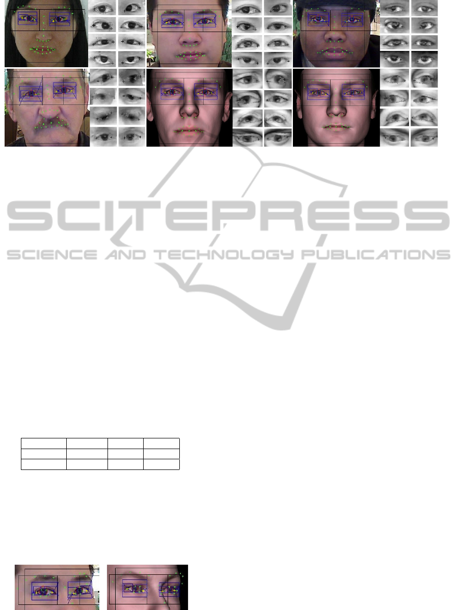
Figure 6: Real and synthetic test sequences.
4.2 2D/3D Eye Corner Detection
This sections evaluates the precision of the eye cor-
ners calculated by the 3D CLM model, our 3D eye
corner detector and its 2D variant. In the latter case
we simply fixed the (rotation) parameters of our 3D
eye corner detector to zero in order to mimic continu-
ous frontal head pose.
To measure the eye corner detection accuracy, we
used 100 BFM-based video sequences . Thus, the
ground-truth 2D eye corner coordinates were avail-
able during our tests.
The eye corner detection accuracy we calculated
as the average least square error between the ground-
truth and the calculated eye corners of each image of a
sequence. The final results displayed in Table 1 show
the average accuracy for all the sequences in pixels
and the improvement percentage w.r.t the 3D CLM
error.
Table 1: Comparison of the 3D CLM, and the 2D/3D eye
corner (EC) detector.
Type 3DCLM 2DEC 3DEC
Accuracy 0.5214 0.4201 0.4163
Improve 0.0 19.42 20.15
The results show that the 3D eye corner detection
method performs the best on the test sequence. It is
also shown that both the 2D and the 3D eye corner
detectors outperform the CLM method. This is due
to the fact that our 3D CLM model is sensitive to ex-
treme head pose and it tends to fail in the eye region.
An illustration of the problem is displayed in Figure 7.
Figure 7: CLM fitting failure (green markers around eye
and eyebrow regions) at extreme head poses.
4.3 Non-rigid Reconstruction
In this section we evaluate the accuracy of the non-
rigid and symmetric reconstruction. For our measure-
ments, we use the same synthetic database as in Sec-
tion 4.2. The basis of the comparison is a special fea-
ture set. This feature set consists of the points tracked
by our 3D CLM model. However, due to the eye
region inaccuracy described in Section 4.2, we drop
the eye points (two eye corners and four more points
around the iris and eyelid contour intersections) and
use the eye corners computed by our 3D eye corner
detector.
The non-rigid reconstruction yields the refined
cameras and the refined 2D and 3D feature coordi-
nates of each image of a sequence. The head pose can
be extracted from the cameras. We selected the head
pose and the 2D and 3D error as an indicator of the
reconstruction quality. The ground-truth head pose,
2D and 3D feature coordinates are acquired from the
BFM.
We calculated the head pose error as the average
least square error between the ground-truth head pose
and the calculated head pose of each image of a se-
quence. The 2D and 3D error we define as the average
registration error (Arun et al., 1987) of the central-
ized and normalized ground truth and the computed
2D and 3D point sets of each image of the sequence.
The compared methods are the 3D CLM, our non-
rigid and symmetric reconstruction and its generic
non-rigid variant (symmetry constraint not enforced).
The results displayed in Table 2 show the aver-
age accuracy for all the test sequences in degrees and
the improvement percentage w.r.t the 3D CLM model.
The generic (Gen) and the symmetric (Sym) recon-
struction methods have been evaluated with different
number of non-rigid components (K) as well.
It is seen that by optimizing a huge amount of
parameters, lower reprojection error values can be
VISAPP2014-InternationalConferenceonComputerVisionTheoryandApplications
624

Table 2: Comparison of the 3D CLM, the symmetric and non-rigid and the generic non-rigid reconstruction.
Type 3DCLM Gen (K=1) Gen (K=5) Gen (K=10) Sym (K=1) Sym (K=5) Sym (K=10)
2D Err. 2.73162 2.72951 2.77952 2.78255 2.72853 2.72853 2.72853
2D Impr. 0.0 0.0772 -1.7535 -1.8644 0.1131 0.1131 0.1131
3D Err. 1.03933 0.89338 4.56524 2.50865 0.880928 0.880915 0.880910
3D Impr. 0.0 14.0427 -339.24 -141.37 15.2407 15.2420 15.2425
Pose Err. 0.3443 0.2756 0.5317 0.5974 0.2829 0.2807 0.2908
Pose Impr. 0.0 19.9535 -54.429 -73.5115 17.8332 18.4722 15.5387
reached, however, without the symmetry constraint
this can yield an invalid solution. Our proposed sym-
metric method keeps stable even with a high number
of non-rigid components (K).
One can also see that the head pose error of our
proposed method outperforms the 3D CLM, however,
the generic rigid reconstruction (Gen (K=1)) provides
the best results. We believe that the rigid model can
better fit to the CLM features due to the lack of the
symmetry constraint.
On the other hand the best 3D registration errors
are provided by our proposed method. It shows again
that the symmetry constraint does not allow the re-
construction to converge toward a solution with less
reprojection error, but with a deviated 3D structure.
The table also shows that the 2D registration is
best by our proposed method, however, the gain is
very little and the performance of the methods are ba-
sically similar.
5 CONCLUSIONS
It has been shown in this study that the precision of
the human face pose estimation can be significantly
enhanced if the symmetric (anatomical) property of
the face is considered. The novelty of this paper is
twofold: we have proposed here an improved eye
corner detector as well as a novel non-rigid SfM al-
gorithm for quasi-symmetric objects. The methods
are validated on both real and rendered image se-
quences. The synthetic test were generated by the
basel face model, therefore, ground truth data have
been available for evaluating both our eye corner de-
tector and non-rigid and symmetric SfM algorithms.
The test results have convinced us that the proposed
methods outperforms the compared ones and a precise
head pose estimation is possible for real web-cam se-
quences even if the head is rotated by large angles.
REFERENCES
Arun, K. S., Huang, T. S., and Blostein, S. D. (1987). Least-
squares fitting of two 3-D point sets. PAMI, 9(5):698–
700.
Cootes, T., Taylor, C., Cooper, D. H., and Graham, J.
(1992). Training models of shape from sets of exam-
ples. In BMVC, pages 9–18.
Cootes, T. F., Edwards, G. J., and Taylor, C. J. (1998). Ac-
tive appearance models. In PAMI, pages 484–498.
Springer.
Cristinacce, D. and Cootes, T. F. (2006). Feature detection
and tracking with constrained local models. In BMVC,
pages 929–938.
Hajder, L., Pernek,
´
A., and Kaz
´
o, C. (2011). Weak-
perspective structure from motion by fast alternation.
The Visual Computer, 27(5):387–399.
Harris, C. and Stephens, M. (1988). A combined corner
and edge detector. In Fourth Alvey Vision Conference,
pages 147–151.
Hartley, R. I. and Zisserman, A. (2003). Multiple View Ge-
ometry in Computer Vision. Cambridge University
Press.
He, Z., Tan, T., Sun, Z., and Qiu, X. (2009). Towards ac-
curate and fast iris segmentation for iris biometrics.
PAMI, 31(9):1670–1684.
Jank
´
o, Z. and Hajder, L. (2012). Improving human-
computer interaction by gaze tracking. In Cognitive
Infocommunications, pages 155–160.
Matthews, I. and Baker, S. (2004). Active appearance mod-
els revisited. IJCV, 60(2):135–164.
P. Paysan and R. Knothe and B. Amberg and S. Romdhani
and T. Vetter (2009). A 3D Face Model for Pose and
Illumination Invariant Face Recognition. AVSS.
Pernek,
´
A., Hajder, L., and Kaz
´
o, C. (2008). Metric recon-
struction with missing data under weak perspective. In
BMVC. British Machine Vision Association.
Santos, G. M. M. and Proenc¸a, H. (2011). A robust eye-
corner detection method for real-world data. In IJCB,
pages 1–7. IEEE.
Saragih, J. M., Lucey, S., and Cohn, J. (2009). Face align-
ment through subspace constrained mean-shifts. In
ICCV.
Tan, T., He, Z., and Sun, Z. (2010). Efficient and robust
segmentation of noisy iris images for non-cooperative
iris recognition. IVC, 28(2):223–230.
Tomasi, C. and Kanade, T. (1992). Shape and Motion from
Image Streams under orthography: A factorization ap-
proach. IJCV, 9:137–154.
Viola, P. and Jones, M. (2001). Rapid object detection using
a boosted cascade of simple features. CVPR, 1:I–511–
I–518 vol.1.
Wang, Y., Lucey, S., and Cohn, J. (2008). Enforcing con-
vexity for improved alignment with constrained local
models. In CVPR.
Xiao, J., Chai, J.-X., and Kanade, T. (2004). A Closed-Form
Solution to Non-rigid Shape and Motion Recovery. In
ECCV, pages 573–587.
Precise3DPoseEstimationofHumanFaces
625
