Topological Space Partition for Fast Ray Tracing in Architectural Models
Maxime Maria, S´ebastien Horna and Lilian Aveneau
University of Poitiers, XLIM-SIC, UMR7252 CNRS, Futuroscope Chasseneuil Cedex, Poitiers, France
Keywords:
Interactive Ray Tracing, Beam Tracing, Acceleration Structure, Architecture, Topology, Cells-and-Portals.
Abstract:
Fast ray-tracing requires an efficient acceleration structure. For architectural environment, the most famous is
the cells-and-portals one. Many previous works attempt to automatically construct a good cells-and-portals.
We propose a new acceleration structure which extends the classical cells-and-portals. It is automatically
extracted from the topological model of a given building. It contains a low number of large volumes, all
of them linked into a graph model. The scan of our structure is particularly simple and rapid, using all the
topological information available from the topological model. The scan can be done for a single ray, or a wide
ray packet. We show in this paper that our structure allows an interactive rendering even for large building
models, with direct lighting from some thousands of point lights.
1 INTRODUCTION
Ray-tracing is a rendering technique allowing to com-
pute high-quality realistic images. It allows to render
all kinds of visual phenomena such as reflection, re-
fraction, direct or global illumination. Its main dis-
advantage lies in its high computational cost. In-
deed, for each pixel to render, at least one ray is cast
through a virtual scene. This simulates the light trans-
port through the scene, and returns the color of the
pixel. For a given ray, the problem consists in find-
ing the nearest intersection, among the geometry of
the scene. From Whitted’s work (Whitted, 1980) to
nowadays, many methods have been proposed to im-
prove ray tracing efficiency. Usually, a well-suited
acceleration structure is used to reduce the number of
useless ray intersection tests.
As part of architectural environments, lighting
simulation can be useful, for instance to visualise a
building before its construction. General accelera-
tion structures such as kd-trees (Bentley, 1975), BSP-
trees (Fuchs et al., 1980), regular grids (Fujimoto
et al., 1988) or bounding volume hierarchy (Rubin
and Whitted, 1980; Kay and Kajiya, 1986) are not
fully adapted to architectural scenes. While they can
be used for a broad range of applications, they can
produce bad rendering results, particularly with archi-
tectural scenes.
Usually, buildings are rendered using a specific
acceleration structure, called cells-and-portals. In
previous works (Airey et al., 1990; Teller et al., 1994;
Meneveaux et al., 1998; Fradin et al., 2005), the ef-
ficiency of cells-and-portals have been demonstrated
using only neighbourhood information between vol-
umes.
In this article, we propose a new acceleration
structure for ray tracing in architectural environments.
This structure consists in a topological model corre-
sponding to a 3 dimensional space partition. It ben-
efits from all topological information available, i.e.
neighbourhood relations between volumes (as in pre-
vious works), and also between faces, edges and ver-
tices. This new structure is well-suited for ray casting
purpose, ray tracing with reflection, refraction and di-
rect or global illumination. It comes with an efficient
beam traversal algorithm, that uses all the topologi-
cal relations to schedule and speed up ray intersection
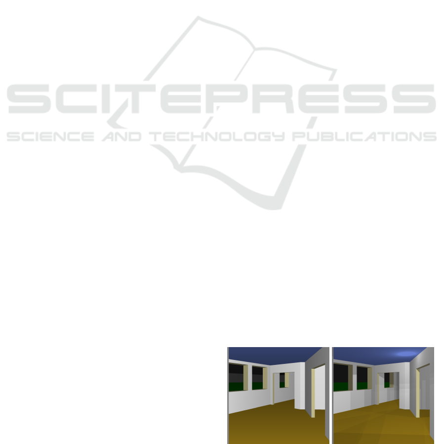
(a) Ray casting, 375 FPS (b) Direct lighting, 22 FPS
Figure 1: Examples of rendering in a building made up of
30k polygons, for 1024× 1024 pixels without anti-aliasing.
Left corresponds to a packet ray casting, right illustrates
direct lighting from the 199 ponctual light sources in that
scene.
225
Maria M., Horna S. and Aveneau L..
Topological Space Partition for Fast Ray Tracing in Architectural Models.
DOI: 10.5220/0004720402250235
In Proceedings of the 9th International Conference on Computer Graphics Theory and Applications (GRAPP-2014), pages 225-235
ISBN: 978-989-758-002-4
Copyright
c
2014 SCITEPRESS (Science and Technology Publications, Lda.)
tests. Using this topological information, a simple
calculation associates each cell with a list of poten-
tially visible light sources. Thus, our structure traver-
sal leads to interactive frame rates using ray tracing,
even for scenes containing many light sources (cf.
Figure 1).
This paper is organised as follows: Section 2 re-
views previous works on acceleration structure for ray
tracing in general and then specifically focuses on
those dedicated to architectural environments. Sec-
tion 3 introduces our topological acceleration struc-
ture. Section 4 presents our topological strategy used
to accelerate the traversal of one ray through the
scene. Section 5 extends the traversal of our structure
for reflection and lighting, as examples of its capabil-
ities. Section 6 gives and analyses some ray-tracing
results. At last, Section 7 concludes and gives some
future work lines.
2 RELATED WORKS
Since 1968 and Appel’s works (Appel, 1968), ray
tracing has been used to compute high quality realistic
images (Whitted, 1980; Cook et al., 1984; Glassner,
1989) including reflection and refraction phenomena
or global illumination account. While the first interac-
tive ray tracer was proposed by Parker et al. in (Parker
et al., 1999) using a large shared memory supercom-
puter, interactive frame rates rendering using ray trac-
ing still remains a non trivial task. Most of the time,
an acceleration structure is built over the scene in
order to improve ray tracing performances. In this
section, we briefly present the common acceleration
structures. Then, we focus on structures dedicated to
the architectural environments.
2.1 General Acceleration Structures
A naive approach of tracing a ray through a scene
would consist in testing the intersection between rays
and all the polygons making up the scene. For interac-
tive rendering, such an approach is obviously prohib-
ited. An acceleration structure is designed to decrease
this linear complexity. It relies on a special organisa-
tion of the geometry which aims to speed up a ran-
dom access to a polygon to a logarithmic time. As a
consequence, the number of ray intersection tests per-
formed is highly reduced and the rendering is faster.
Many acceleration structures have been proposed in
the literature such as kd-trees (Bentley, 1975), bound-
ing volume hierarchies (BVH) (Rubin and Whitted,
1980; Kay and Kajiya, 1986) or regular grids (Fuji-
moto et al., 1988). A survey comparing all these ac-
celeration structures on CPU can be found in (Havran,
2000).
These structures are general, in that they work
with any kind of scenes. Nevertheless, in some cases
their traversal cost can become very high. That is
the case for architectural environments. First, build-
ings can contain little but highly detailed objects in-
side big empty spaces. This kind of configuration is
well known as the ”teapot in the stadium” problem. It
slows down traversal performances of regular struc-
tures like regular grids. A second problem appears
with architectural environments with walls in general
configurations. With axis-aligned partitioning meth-
ods, such as kd-tree or BVH, the cutting splits do not
respect the wall positions and produce a complex sub-
division scheme. These two problems explain for the
most part why general acceleration structures are not
favoured to render architectural scenes.
2.2 Architectural Acceleration
Structures
Architectural scenes are made up of large occlusive
surfaces such as floors, ceilings or walls. From a
given point of view only a small part of the scene is
visible. The structure called cells-and-portals takes
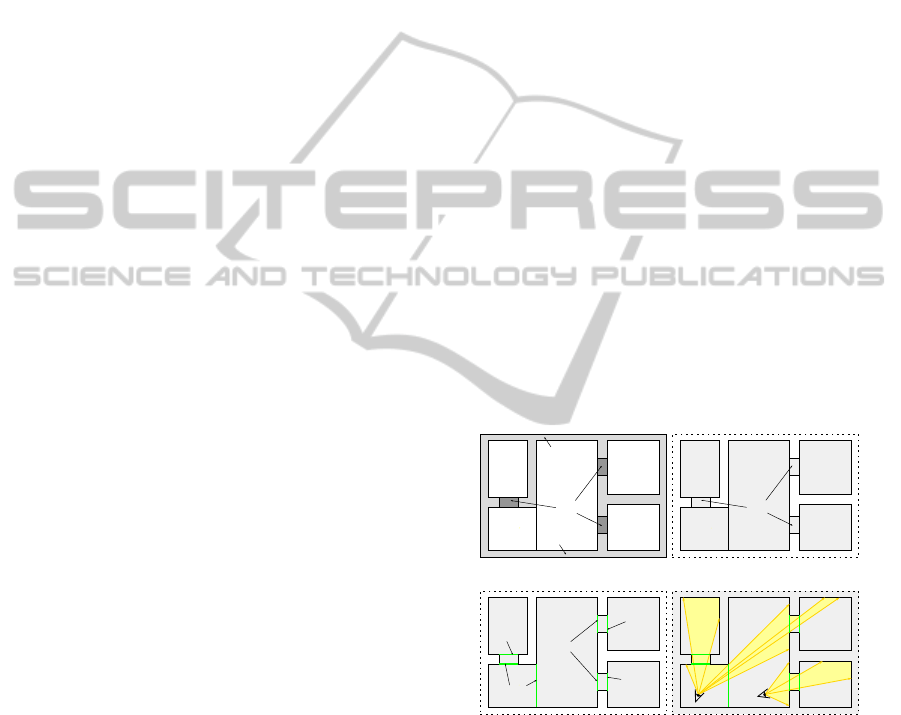
advantage of this particular structural organisation.
Room
Doors
Wall
Wall
Room
Room
Room
Room
(a)
Cell
Cell
Cell
Cell
Cell
Cells
(b)
Portal
Portals
Portals
Portal
Portal
(c) (d)
Figure 2: 2D cells and portals representation and usage:
(a) building representation; (b) rooms and doors correspond
to cells; (c) portals are shared by 2 cells; (d) rays hitting a
portal are propagated through neighbouring cells.
In such a structure, a cell represents a volume in
which light can be propagated, such as a room or an
opening. A portal corresponds to a face incident to
two cells (cf. Figure 2). A cells-and-portals is stored
in a graph, where a node represents a cell and an edge
corresponds to a portal. The principle of traversal
consists in scanning such a graph. From a given cell
C, a ray r can exist only by a face incident to C. If this
GRAPP2014-InternationalConferenceonComputerGraphicsTheoryandApplications
226

outgoing face is a portal, then r is propagated in the
neighbouring cell; else it is stopped (cf. Figure 2(d)).
Due to the local complexity of this process, it remains
efficient even for large architectural scenes.
Several methods have been proposed to construct
such a structure starting from a list of polygons. Airey
et al. (Airey et al., 1990) described a method for ar-
chitectural scenes with axis-aligned walls. The sub-
division is performed using a kd-tree. It has been
extended for general convex cells (non necessarily
axis-aligned) using a BSP-tree by Teller et al. (Teller
and S´equin, 1991). Meneveaux et al. (Meneveaux
et al., 1998) used a rule-based system which consists
in finding the openings (i.e. the portals), in order to
use them to construct cells that fit better with walls.
All these works aim at extracting neighbourhood in-
formation between volumes. The problem of these
methods is that the cells are not optimally determined
so that a room could be uselessly split several times.
In (Fradin et al., 2005), cells-and-portals are
directly extracted from architectural environments
which are built by using a dedicated topological mod-
eller. Resulting scenes are adapted for lighting sim-
ulation in large buildings as shown in (Fradin et al.,
2005; Fradin et al., 2006). Neighbourhood informa-
tion between volumes are directly known from the
topology. This work produces an optimal cells-and-
portals structure in which a room is represented by an
unique cell. Nevertheless, it has two main drawbacks.
Firstly, the full potential of the topological model is
not exploited: Indeed, the neighbourhood relations
between faces, edges and vertices are known but un-
used. Secondly, the construction is entirely manual so
that designing a scene is a long and tedious task. In
addition, scenes can not be validated when no archi-
tectural constraints or editing operations are provided.
In this paper, we use the model introduced by
Horna et al. in (Horna et al., 2009). It is also a
topological model, but it can produce automatically
the piece of information needed to cell-and-portals
traversal. This model is described in more details in
Section 3. The associated modeller allows to auto-
matically generate the 3 dimensional structure from
an architectural plan (Horna et al., 2007). Moreover,
contrary to Fradin et al. we propose to exploit all
its topological properties, leading to a very efficient
traversal.
3 TOPOLOGICAL STRUCTURE
In this section, we present our topological accelera-
tion structure for architectural environments.
3.1 Generalized Maps
An architectural environment can be considered as a
set of volumes. Each volume corresponds to a unique
element in the scene (room, wall, door, window, etc.).
Therefore, an adjacency graph is sufficient to store
such a structure.
Our acceleration structure is based on the topolog-
ical model introduced by Horna et al. (Horna et al.,
2009). It uses the notion of topological dimension,
which is associated with geometrical objects: Dimen-
sion 3 with a volume, dimension 2 with a face, di-
mension 1 with an edge and dimension 0 with a ver-
tex. This model contains topological relations be-
tween all these geometric elements, from dimension
0 to 3. It is based on generalized maps, or G-maps
(Lienhardt, 1994), extended by the formal definition
of a set of topological, geometrical and semantic con-
straints specifically dedicated to architectural mod-
elling. These constraints ensure the model validity
during all the modelling process.
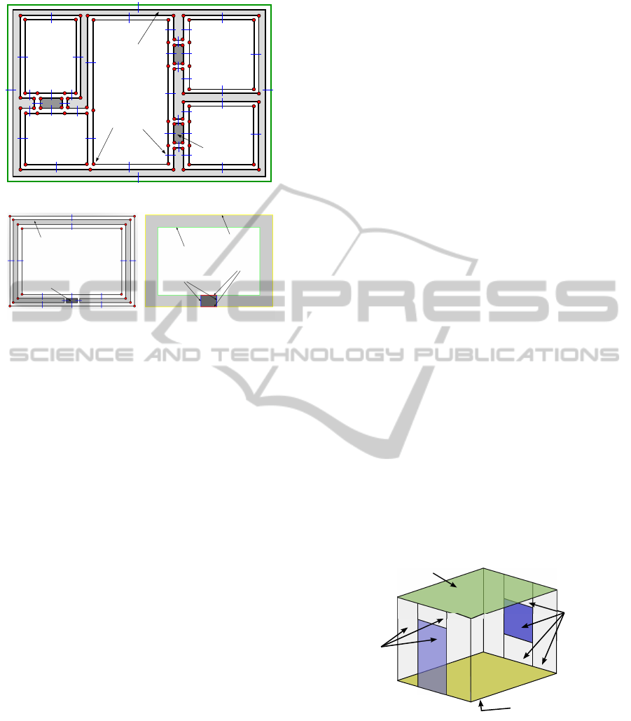
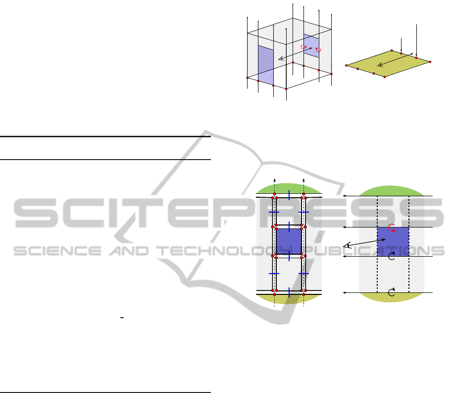
E
2
E
1
1D link
Face
(a)
F
2
F
1
2D link
(b)
V
1
V
2
3D link
(c)
Figure 3: Topological links in each dimension: (a) links of
dimension 1 bind edges to make faces; (b) links of dimen-
sion 2 tie together faces to generate volumes; (c) volumes
are tied with links of dimension 3.
In an architectural environment, all elements are
real world objects. In such a scene, two elements can
not occupy the same space, and the whole space is
filled, authorizing a space partition. Consequently,
topologically speaking, a building should be defined
as a subdivision of space into volumes, faces, edges
and vertices. In this article, we only recall the main
principles of generalized maps applied to buildings,
i.e. the neighbourhood information. All the defi-
nitions and properties of n-dimensional generalized
maps can be found in (Lienhardt, 1994). The Fig-
ure 3 shows how topological information is organised
(for simplification, links of dimension 0, binding two
vertices to make an edge, are not represented).
3.2 Architectural Topological Model
Architectural scenes are represented by a 3 dimen-
sional oriented and closed space subdivision com-
posed of elements with a significant thickness. Each
TopologicalSpacePartitionforFastRayTracinginArchitecturalModels
227
Exterior
Neighborhood
Room
Wall
relations
Room
Room
Door
Room
(a)
EXTERIOR
DOOR
WALL
ROOM
WALLPAPER
FACADE
GATE-POST
PORTAL
(b)
Figure 4: Topology and semantic: (a) 2 dimensional scene
complying the topological and semantic properties; each
face (in 3D, each volume) corresponds to a unique element
(room, wall, etc.); topology represents neighbouring rela-
tions. (b) An edge (in 3D, a face) incident to two cells
becomes a PORTAL while a non-portal edge has a specific
semantics (WALLPAPER, FACADE, GATE-POST).
volume is identified by a unique semantic according
to its nature: ROOM, DOOR, WALL, GROUND, CEIL-
ING or EXTERIOR. The Figure 4(a) illustrates a scene
complying to this property. Note that all descriptions
made in dimension 2 are extensible to dimension 3,
since G-maps are homogeneous in all dimensions.
From this model, we design a cells-and-portals
structure in the following way: In the cells-and-
portals philosophy, a cell is a volume where light can
be propagated. This corresponds to a given subset of
semantic: ROOM, DOOR, EXTERIOR. Then, with our
architectural model, the cells can be deduced auto-
matically from the volumes.
In the same manner, a portal is a face which can
be crossed by the light. With our model, portals are
automatically deduced from semantics. Indeed, the
only way to stop the light is to find a non cell volume.
Then, using the semantic information stored into our
structure, a face is a portal if and only if it links two
cells (cf. Figure 4(b)).
In fact, our model is also used to find automati-
cally the semantics of each face, even the non portal
one. This allows to deduce the reflecting properties of
non portal faces, and is exploited during the render-
ing. For example, a face incident to a ROOM and a
WALL is identified as a WALLPAPER, while one inci-
dent to a DOOR and a WALL becomes a GATE-POST.
3.3 Our Acceleration Structure
Architectural environments are mostly composed of
rooms made with large vertical planes for the walls,
and horizontal planes for floor and ceiling. Hence, we
represent each volume by two horizontal faces (upper
and lower ones) and a set of vertical bounding faces.
Each vertical face can be divided into several ver-
tical parts, eg. to represent a door or a window (cf.
Figure 5).
Our structure results in a space partition, repre-
senting a cells-and-portals structure in which a cell
corresponds to an unique room. Nevertheless, for ren-
dering efficiency our structure traversal is optimised
for convex cells. Then, each concave cell is automat-
ically subdivided into a set of convex cells (sharing
portals). Thus, finally, a room is made of several cells.
Our acceleration structure is stored into a compact
graph structure. A node corresponds to a cell and the
graph links are the topological links of dimension 3
(the neighbourhood between cells i.e. the portals).
Each node (so cell) contains its 2 dimensional lower
face made of vertices. It is ordered counter clockwise
(i.e. from right to left from inside the volume). Each
vertex contains a list of horizontal edges representing
the vertical faces, with their semantics. It is ordered
from the bottom up. At least, a node contains a ceil-
ing height. This particular data structure (organised
according to topological elements) allows to sched-
ule and then to speed up the traversal process. Next
section describes the traversal algorithm for one ray.
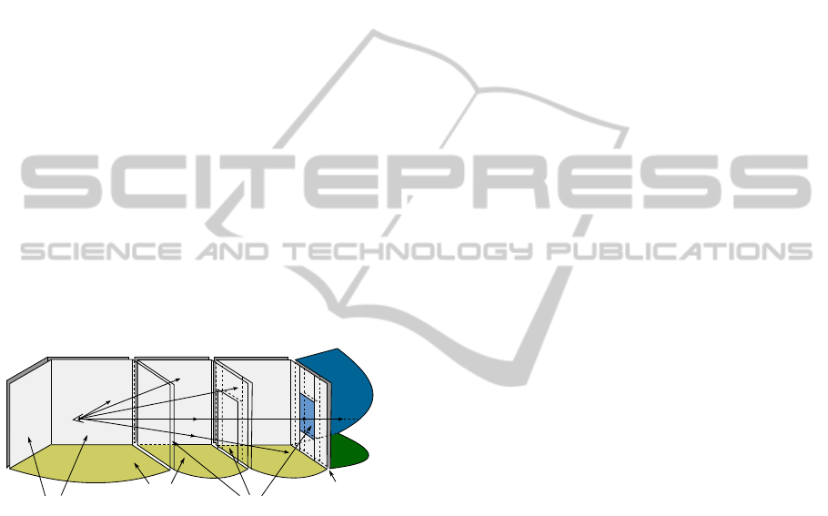
Lower face
Vertical
Upper face
faces
Vertical
faces
Figure 5: Volume characteristics in building: They are com-
posed of 2 horizontal faces and several vertical faces corre-
sponding to volume border.
4 STRUCTURE TRAVERSAL
The traversal of our structure requires displacement
in a graph. In fact, it consists in a classical cells-
GRAPP2014-InternationalConferenceonComputerGraphicsTheoryandApplications
228
and-portals traversal but improved by using available
topological links in all dimensions.
In this section, we firstly present the principle of
a basic ray casting in our topological structure. Then,
we recall the Pl¨ucker coordinates, which are used for
intersection tests. Finally, we explain our topological
strategy use to improve the outgoing face search.
4.1 Basic Ray Casting
Without considering the optimisation brought by our
topological strategy for the outgoing face search, our
acceleration structure is a kind of cells-and-portals.
Then, a basic ray casting is a straightforward prob-
lem. All the rays are propagated through the scene
starting from the volume containing the camera. Nev-
ertheless, this algorithm hides two key points.
The first on resides in the determination of the ini-
tial volume (or camera volume). This volume is cal-
culated once and only once. Then, when the cam-
era is moved by the user, the camera volume is up-
dated according to the translation vector defining the
movement; this costs nothing since it simply consists
in casting a finite and short ray. Thus, the updated
camera volume corresponds to the ray arrival volume.
V
1
: ROOM 1
r
1
V
2
: ROOM 2 V
3
: ROOM 3
V
4
: EXTERIOR
WALLPAPER
r
2
r
3
r
4
r
5
GROUND
PORTAL
FACADE
Figure 6: Scene traversal: Rays start from volume V
1
and
are propagated when they hit a face PORTAL, or are stopped
when they hit a boundary face (WALLPAPER, GROUND,
etc.). As an example, ray r
1
hits a face in V
1
with seman-
tics WALLPAPER, while ray r
4
goes through three portals
before being propagated inside volumeV
4
of semantics EX-
TERIOR.
The second key point lies in finding the outgoing
face of a given ray in a given volume. If this face
has a semantics PORTAL, then the ray is propagated
through its neighbouring volume by using topological
relation of dimension 3. Else, the hit face is a bound-
ary face (semantics WALLPAPER, GROUND, etc.) and
the ray is stopped (cf. Figure 6).
As mentioned in Section 2.2, the global number of
faces making up the scene does not really matter due
to the local complexity of the traversal. Given that the
propagation of a ray from a volume to its neighbour
is constant by using topological relation of dimension
3 (i.e. volume neighbouring), the efficiency of such
an algorithm lies in finding quickly the outgoing face
of a given ray inside a volume. To improve that and
thus the global traversal, we propose an outgoing face
search scheduling based on the topology of the scene.
While previous works only used neighbouring rela-
tion between volumes (of dimension 3), we also use
relation between faces (dimension 2), edges (dimen-
sion 1) and vertexes (dimension 0), in order to speed
up the outgoing face search. Section 4.3 explains in
details this process.
4.2 Pl
¨
ucker Coordinates
Pl¨ucker coordinates was firstly introduced in (Pl¨ucker,
1865). Generally speaking, they are used to represent
linear subspaces of dimension k in a projective space
of dimension n. In computer graphics, they represent
oriented lines of 3 dimensional geometrical space.
They are particular point in the projective 5 dimen-
sional space P
5
. More precisely, an oriented line l de-
fined by two distinct points A and B is represented by
a sextuplet of coordinates Π
l
= {u= b−a: v = a×b},
where the 3 dimensional vectors a and b are respec-
tively the position of the points A and B. Hence, the
vector u corresponds to the direction of the line, while
v is its position (or its mechanical moment).
As a example of Pl¨ucker coordinates useful-
ness, they are used in visibility problems as shown
in (Teller and Hanrahan, 1993; Charneau et al., 2007;
Fang, 2010; Mora et al., 2012). Here, we use them to
determinate the relative orientation between two ori-
ented lines via the operator side (Shoemake, 1998).
This operator is defined for two lines l and l
′
as
side(Π
l
, Π
l
′
) = u.v
′
+ u
′
.v. If the result is negative,
l turns clockwise around l
′
; if it is positive, l turns
in the counterclockwise around l
′
; else, when side is
null, the two lines have a common point (in fact they
are coplanar, and so they meet at least at infinity).
4.3 Outgoing Face Search
Using the topological relations available in our struc-
ture, we develop a simple and efficient algorithm for
searching the outgoing face of a given ray into a vol-
ume (cf. Algorithm 1). It is divided into two main
steps.
Let us recall that each volume is convex. Then
a ray can only exit through an unique face. First,
we consider the volume as an infinite vertical polyhe-
dron, ignoring the upper and lower faces. Therefore,
we start to search the outgoing infinite vertical section
(Algorithm 1 - line 3-7).
An infinite vertical section is bounded by two ver-
tical lines oriented from the bottom up. Using Pl¨ucker
TopologicalSpacePartitionforFastRayTracinginArchitecturalModels
229
lines, it is trivial to test if a ray exits through a given
vertical section, by testing its side product with the
two bounding lines. Indeed, a ray intersects such a
section when it goes through the left (resp. right) of
the right (resp. left) line. This search is done lin-
early, by scanning the vertices of the lower face. It
uses both topological relations of dimension 1 and 0
(i.e. links between edges and vertices). Considering
the low number of vertical sections per volume (in av-
erage 4.37) a more complex scan (like dichotomy) is
useless.
Algorithm 1: Outgoing face search for a given ray r
into a volume V.
Require: V: volume; r: ray;
1: {First step: search the outgoing vertical section}
2: i ⇐ 0;
3: while (sideVertical(r, V.vSec[i].left) ≤ 0
k sideVertical(r, V.vSec[i].right) > 0) do
4: i ⇐ i+ 1;
5: end while
6: {Second step: search the outgoing face in the
vertical section i}
7: h ⇐ V.vSec[i].hSec[];
8: if sideHorizontal(r, h[0]) < 0 then
9: return h[0]; {go through the floor}
10: end if
11: for k = 1 to V.walls[i].nb
hSec−1 do
12: if sideHorizontal(r, e[k]) < 0 then
13: return e[k];
14: end if
15: end for
16: {Not a regular face: outgoing face is the ceiling!}
17: return V.ceiling;
It should be noticed that this first step is done
strictly in dimension 2 (see Figure 7). If x and y are
the 2D coordinates of a line bounding the wall (with
direction u = z), and for a ray defined with Pl¨ucker
coordinates Π
l
= {π
0
, π
1
, π
2
, π
3
, π
4
, π
5
}, then the side
operator is reduced to: y× π
0
− x × π
1
+ π
5
.
Once the outgoing infinite vertical section is
found, we search for the outgoing face. We consider
the outgoing vertical section as a set of infinite faces
bounded by two horizontal lines (see Figure 8). Let us
recall that these lines are oriented from right to left in
our acceleration structure. Then we can use Pl¨ucker
side product to test the ray intersection. We start from
the lower edge (Algorithm 1 - line 9-12): If the result
is negative, the ray turns clockwise around the edge
(the ray goes below the edge); then the floor is hit and
can be returned. Otherwise, we repeat this process
with upper edges by scanning them (by using topo-
logical relations of dimension 2, i.e. links between
1
2
3
4
5
7
8
6
l
1
l
2
r
(a)
1
2
3
4
5
8
6
l
1
= (a
1
, b
1
)
l
2
= (a
2
, b
2
)
7
r
(b)
Figure 7: First step of outgoing face search: (a) the cell
is considered as an infinite vertical polyhedron; a vertical
section is bounded by two lines oriented from the bottom
up; outgoing vertical section is 6; (b) the process is strictly
done in 2D.
E
D
C
B
A
(a)
E
C
A
B
D
l
3
r
l
2
l
1
l
4
(b)
Figure 8: Second step of outgoing face search: (a) a ver-
tical section is divided into several faces, including ground
and ceiling; (b) a face is bounded by two horizontal lines
oriented from right to left; outgoing face is C.
faces) until finding the outgoing face (Algorithm 1 -
line 13-17). If none face is found, then the ceiling is
returned (Algorithm 1 - line 18). Once more, a non-
linear strategy is useless in front of the low number
of faces (in average 2.11). Considering that bound-
ing lines are only horizontal, Pl¨ucker side operator is
reduced to four products and five additions.
To sum up, outgoing face search is optimised by
using topological relations of all dimensions:
• Dimensions 0 (vertex) and 1 (edge) to scan the
lower face of a volume and to find the outgoing
vertical section.
• Dimension 2 (face) to change of face within a ver-
tical section and determine the outgoing face.
• Dimension 3 (volume) to move from a volume to
its neighbour when propagating a ray.
GRAPP2014-InternationalConferenceonComputerGraphicsTheoryandApplications
230
5 EXTENDED USES
This section discusses about the integration of our
model into a ray tracing application to render archi-
tectural scenes, using wide ray packets and secondary
rays (reflection, refraction, and light rays).
5.1 Ray Packet
The basic ray casting algorithm is modified in order to
group the rays in packets. In practice, we use can very
wide packet: depending on the number t
h
of threads,
we divide the image into 2 × t
h
packets. In our ex-
periments, this leads to 16 packets for 1024 × 1024
pixels.
A packet is defined by its 4 corners, correspond-
ing to 4 pixels in the ray casting (and idem for sec-
ondary rays). From the initial volume, the outgoing
face of this 4 rays is searched according to Algorithm
1. When the results are coherent (the 4 rays goes
through the same face), the algorithm computes suc-
cessfully the outgoing face for all internal rays.
Else, when rays are incoherent, the algorithm can
not continue for the given packet. For each corner
rays, all the current data is stored: i.e. the identifiers
of the volume, of the vertical section and of the face
of this vertical section. Then, the packet is split in
2 or 4 parts, depending on the incoherence and each
part continue in the same way, from the same initial
position.
In practice, this strategy is very efficient. It uses
SIMD float point instruction as, for instance, in the
kd-tree packet traversal proposed in (Wald et al.,
2001). Since the new packets continue from where
they are split we do not spend time in a new structure
scanning.
5.2 Reflection and Refraction
Our model allows to associate any kind of behaviour
to a face thanks to the face semantics. This allows
to add some reflection or refraction properties to the
surfaces, as an example for panes.
When a ray hit a reflective or refractive surface,
its trajectory is modified. For a both reflective and
refractive surface, it is also subdivided. Since our
traversal algorithm have a local scope, the cost of a re-
flective or refractive ray stays about the same that for
primary rays. For example, with a specular surface, a
ray can be reflected a given number of times. For each
bounce, a new ray have to be cast, with new Pl¨ucker
coordinates. In fact, specularity account is not a diffi-
cult task. The new coordinates of the specular ray are
computed according to a traditional scheme (cf. Sec-
tion 4.2) and the ray is propagated by using the Al-
gorithm 1, or its packet version. The main difference
resides in the starting cell: The volume containing the
reflection point is not the same that the camera one.
Fortunately, this volume do not have to be computed:
It corresponds to the arrival volume of the primary
ray.
5.3 Direct Illumination
Computing the direct illumination is a good way to
evaluate the robustness of our structure in case of spa-
tially incoherent rays. That implies new rays (light
rays) to be cast through the scene, to determine the
point-to-point visibility between the primary ray in-
tersections and the point light sources. Each new ray
is simply cast, as a primary ray (see Section 4). Then,
lighting is computed according to the visibility and
the chromatic intensity of each visible source.
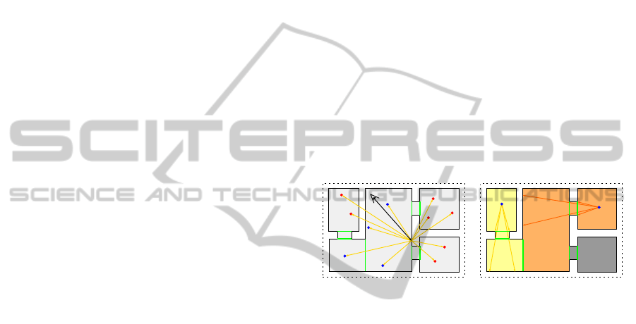
r
(a)
L
1
L
2
(b)
Figure 9: Direct illumination: (a) for the ray r, 11 light
rays are launched while only 4 are visible (in blue); (b) cells
crossed by light beams are potentially illuminated, allowing
to decrease the number of light rays.
The main difficulty for direct illumination account
in architectural environments lies in the huge num-
ber of light sources which highly increase the number
of rays to be cast, leading to low frame rates. For-
tunately, given that buildings are composed of large
occlusive surfaces, too many useless tests are per-
formed (cf. Figure 9(a)). Cells-and-portals structures
are used in (Airey et al., 1990), (Teller and S´equin,
1991), (Luebke and Georges, 1995) or (Meneveaux
et al., 1998) to compute the potentially visible set (or
PVS) in architectural environments. From the same
perspective and for efficiency purpose, we choose to
compute the set of potential visible lights for each cell
making up our scenes. We proceed by launching con-
tinuous beams from a light source, one through each
opening of the volume containing the light source(cf.
Figure 9(b)). Parts of the beam which hit a face POR-
TAL are recursively propagated through neighbouring
cells until being stopped by a non-portal face. As
usual, the propagation is performed by using topolog-
ical relation of dimension 3. Each cell crossed by the
beam is potentially illuminated by the light source.
TopologicalSpacePartitionforFastRayTracinginArchitecturalModels
231
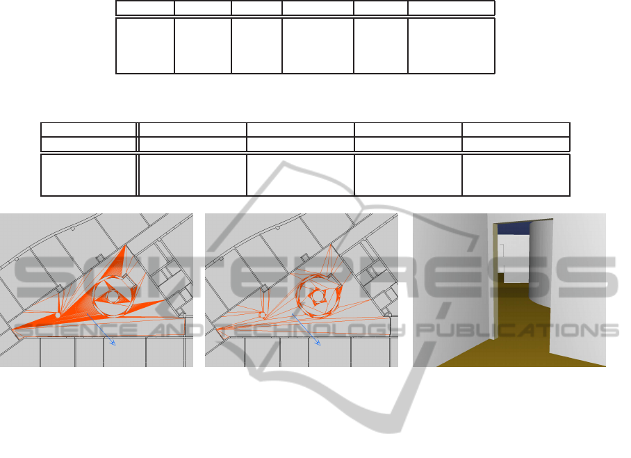
Table 1: Characteristics of our test scenes: number of rooms, cells, polygons, lights and memory size in megabytes.
Scenes # rooms # cells # polygons # lights memory (Mb)
HOUSE 8 509 1.166 8 0.46
BUILD1 46 2.333 8.557 55 2.03
BUILD2 135 8.258 29.937 199 6.82
BUILD3 1755 95.932 369.521 2557 80.13
Table 2: Results: for each scene we give the average number of frame calculated per second (FPS), and the average number
of rays cast per second in millions (Mrays/s).
Scenes HOUSE BUILD1 BUILD2 BUILD3
Results FPS Mrays/s FPS Mrays/s FPS Mrays/s FPS Mrays/s
Ray casting 65.09 68.26 51.28 53.78 51.35 53.85 46.86 49.14
Packet casting 388.16 407.01 384.13 370.68 375.13 393.35 341.66 358.25
Packet Lighting 128.71 419.75 66.64 367.05 60.48 352.09 34.49 246.91
(a) Convexification using (Fern´andez et al.,
2008)’s method; Rays cross 9.139.670 volumes in
all to render the image (c).
(b) Convexification extended with bounding boxes
and topology; Rays cross 3.422.570 volumes in all
to render the image (c).
(c) Associated rendered image; 314,31 FPS with
convexification (a) and 377,28 FPS with (b).
Figure 10: Comparison of the convexification of a room.
Instead of having to cast a light ray for each light
source, computing PVS allows to highly reduce the
number of lights to a local list of potentially visible
sources. As an example, in one of our test scene
which contains 199 light sources, the average num-
ber of light rays per image is reduced from 208.67
millions to 10.14 millions (-95.14%).
6 RESULTS
We evaluate the performances of our acceleration
structure on a Intel
R
Core
TM
i7 CPU 960 @ 3.20GHz
with 12GB of RAM. The traversal algorithm runs
in parallel using OpenMP. The packet version also
uses 4-wide SIMD floating point instructions (Intel
R
SSE). Performances are given in terms of:
• FPS: frames calculated per second.
• Mrays/s: millions of rays cast per second.
The rendering is done for image of 1024× 1024 pix-
els with one ray per pixel (without anti-aliasing). In
order to have relevant statistics, we use a way-point
system to keep the same points of view for each algo-
rithm tested. These points of view result from a walk-
through into each scene; then the number of points of
view can differ according to the size of the scene.
Notice that the rendering time include the shading,
using a Lambertian brdf. With ray-casting, a virtual
point light is positioned at the camera location, and
used for the calculation of the cosine of the incident
direction with respect to the surface normal.
6.1 Scenes
We present four of our test scenes which are more or
less complex in terms of size, number of polygons
and light sources. Their main characteristics are sum-
marised into Table 1. The smallest scene corresponds
to a house made up of 8 rooms (cf. Figure 12). It
has 1.166 polygons and contains 8 light sources. The
scenes BUILD1 and BUILD2 represent two distinct
floors of a large administration building (cf. Figures
13, 1 and 11). They are respectively made up of 46
and 135 rooms, and contains 8.557 and 29.937 poly-
gons with 55 and 199 light sources. The last scene,
BUILD3, is a very large building made up of 13 floors
with 1755 rooms, with 369 thousands of polygons and
2557 point light sources (cf. Figure 14). These four
scenes result directly from our topological modeller.
GRAPP2014-InternationalConferenceonComputerGraphicsTheoryandApplications
232
6.2 Results and Discussion
6.2.1 Primary Ray Casting
We propose two different algorithms for primary ray
casting. While the first one works pixel per pixel, the
second corresponds to the packet traversal described
in Section 5.1. These two algorithms have been eval-
uated with each of our test scenes.
(a) Ray casting (48 FPS). (b) Ray packets (356 FPS).
Figure 11: Illustration of primary ray casing with scene
BUILD2.
We can notice that primary ray casting using our
topological structure is very efficient (see Table 2).
The Figure 11(a) shows the rendering for the second
building test scene, using a simple ray casting. The
Figure 11(b) proposes the same point of view, but us-
ing and emphasizing ray packets. Clearly, the packet
are split only near cell boundaries. For large wall,
ground or ceiling parts, a wide ray packet can be effi-
ciently traced with our acceleration structure.
Table 3 compares the performances of these two
methods with those measured by using the ray trac-
ing kernel Embree (Ernst and Woop, 2011). We can
observe both of them are faster than Embree. Our ray
casting method is more than 4 times faster and the
packet version is more than 30 times faster.
Table 3: Comparison with Embree ray tracing soft-
ware (Ernst and Woop, 2011).
Scenes Embree Ray casting Packet casting
HOUSE 18 65.09 388.16
BUILD1 12 51.28 384.13
BUILD2 10 51.35 375.13
BUILD3 8 46.86 358.25
Since our algorithm have a local complexity, the
size of the scene does not matter since the data could
fit easily on the available memory. This complexity
takes into account the number of volumes crossed by
the ray and the number of polygons making up these
volumes (which impact on the outgoing face search).
Indeed, performances are reduced in case of a cell
split a lot of times or in case of volumes containing
too many polygons (i.e. not enough split). Thus, the
scene must be convexifiedusing a well suited strategy.
Analogous to the well-known surface area heuris-
tic (SAH) (Goldsmith and Salmon, 1987; MacDon-
ald and Booth, 1990), a concave cell have to be split
considering its area and the expected cost of tracing
an infinite random ray through that cell. In fact, we
search for a split scheme which have the lowest SAH
cost possible. The main problem with convexifica-
tion occurs in case of curved walls as illustrated on
Figure 10. The Figure 10(a) shows a room convex-
ified with the method presented in (Fern´andez et al.,
2008). Because of curved walls, many splits are per-
formed, creating a dense partition. Then, rendering
an image requires to cross a lot of volumes so that
performances are highly reduced. Our method is il-
lustrated in Figure 10(b): Convexification is extended
by constructing a bounding box around curved walls
to restraint all the splits in a small space, leading to
a better SAH cost. The use of such a strategy offers
a good compromise and leads to better performances.
Notice that convexification process is automatically
performed with our modeller and takes from seconds
to few minutes according to the size of the scene.
6.2.2 Direct Lighting
Taking into account direct lighting means casting a
light ray for each light source. For one light source
this should twice the number of rays. Then, for x light
sources this can dramatically reduce the number of
frames per second. As explained in Section 5.3, we
compute the PVS for each cell in our structure to re-
duce the number of light rays.
Table 2 shows that direct lighting makes the num-
ber of rays per second drop linearly. Nevertheless,
this reduction is not linear with respect to the number
of light sources. Some rendering examples are pro-
posed in the Figures 1, 12, 13 and 14.
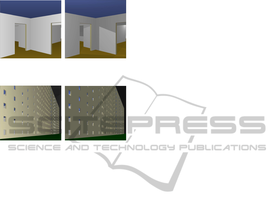
(a) 371 FPS. (b) 75 FPS.
Figure 12: HOUSE without (a) or with (b) lighting from 8
light sources.
This fall in terms of FPS is brought by two causes.
First, new Pl¨ucker coordinates have to be computed
TopologicalSpacePartitionforFastRayTracinginArchitecturalModels
233
(a) 347 FPS. (b) 53 FPS.
Figure 13: BUILD1 without (a) or with (b) direct lighting.
The scene contains 55 light sources.
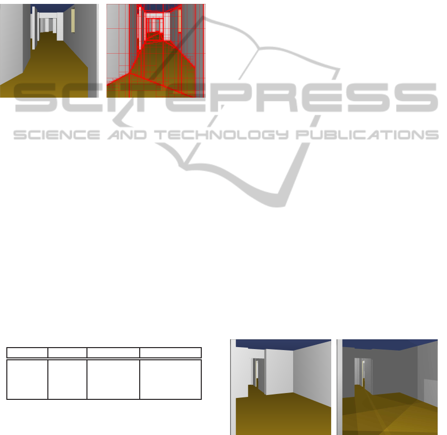
(a) 155 FPS. (b) 0.24 FPS.
Figure 14: BUILD3 without (a) or with (b) direct lighting
from 2557 lights. Most of the lights are visible outside,
leading to a small FPS.
for each light ray to be cast. Secondly, it is due to spa-
tial ray incoherence which leads to incoherent mem-
ory accesses. The robustness of our topological struc-
ture in terms of number of rays cast per second allows
to think that it could be used efficiently to compute
global illumination in architectural environments.
7 CONCLUSIONS
This article proposes a new acceleration structure for
ray tracing dedicated to architectural environments. It
is generated automatically from a topological mod-
eller, without human interaction. It takes advantage of
the architectural building constraint: it corresponds to
a 3 dimensional oriented and closed space subdivision
composed of elements with a significant thickness.
Our structure is a kind of advanced cells-and-
portals, with two main improvements: Firstly, thanks
to our topological model, cells-and-portals cutting
planes fit perfectly to the building topology. Secondly,
while previous cells-and-portals traversal algorithms
used only neighbouring relations between volumes,
we propose to take advantage of all the topological
information available, to schedule the outgoing face
search, and to accelerate the whole process.
The traversal of our acceleration structure is im-
plemented on CPU, both with single rays or with ray
packets. Our experimentation shows that our structure
traversal is very efficient. Our rendering tool com-
putes hundreds of millions of rays per second, using
only a single 4-core processor. Consequently, it al-
lows to render images interactively, for ray casting or
ray tracing, with direct lighting or not.
We think that our structure and its traversal algo-
rithm can run onto a GPU, taking advantage of the
high number of cores. It should be interesting to
study the results of such a structure on GPU, espe-
cially when a large number of light sources are used.
We also think that our structure can be used to in-
clude piece of furniture quite easily. Indeed, using
bounding boxes surrounding high detailed objects, we
should be able to include them into the topological
model. During the rendering step, the rendering could
be done by combining our structure with a more clas-
sical one. Thus, our topological structure traversal
performances would highly depend on the accelera-
tion structure used to render the object.
Then, a logical next step will be to adapt our topo-
logical partition to general objects in order to include
it directly in our architectural structure.
The main disadvantage of our model relies on the
topological modeller. It could not be generated with
only a geometric description of scene, without any
topological information. As a future work, we plan
to adapt our ideas to general objects described only
by their geometry. We aim to use generalized maps
to connect geometric elements themselves, in order
to generate automatically a topological acceleration
structure from scratch, for architectural scenes or not.
This step would allow to directly include furniture in
our architectural structure and thus to avoid the de-
pendence on an auxiliary acceleration structure.
ACKNOWLEDGEMENTS
Authors thanks the R
´
egion Poitou-Charentes for their
funding support.
REFERENCES
Airey, J. M., Rohlf, J. H., and Brooks, Jr., F. P. (1990). To-
wards image realism with interactive update rates in
complex virtual building environments. SIGGRAPH
Comput. Graph., 24(2):41–50.
Appel, A. (1968). Some techniques for shading machine
renderings of solids. In Proceedings of the April
30–May 2, 1968, Spring Joint Computer Conference,
AFIPS ’68 (Spring), pages 37–45. ACM.
GRAPP2014-InternationalConferenceonComputerGraphicsTheoryandApplications
234

Bentley, J. L. (1975). Multidimensional binary search
trees used for associative searching. Commun. ACM,
18(9):509–517.
Charneau, S., Aveneau, L., and Fuchs, L. (2007). Exact,
robust and efficient full visibility computation in the
Pl¨ucker space. Visual Computer, 23(9-11):773–782.
Cook, R. L., Porter, T., and Carpenter, L. (1984). Dis-
tributed ray tracing. SIGGRAPH Comput. Graph.,
18(3):137–145.
Ernst, M. and Woop, S. (2011). Embree: Photo-realistic ray
tracing kernels.
Fang, Q. (2010). Mesh-based Monte Carlo method using
fast ray-tracing in Pl¨ucker coordinates. Biomed. Opt.
Express, 1(1):165–175.
Fern´andez, J., T´oth, B., C´anovas, L., and Pelegr´ın, B.
(2008). A practical algorithm for decomposing polyg-
onal domains into convex polygons by diagonals.
TOP, 16(2):367–387.
Fradin, D., Meneveaux, D., and Horna, S. (2005). Out-of-
core photon-mapping for large buldings. In Proceed-
ings of Eurographics symposium on Rendering.
Fradin, D., Meneveaux, D., and Lienhardt, P. (2006). A
hierarchical topology-based model for handling com-
plex indoor scenes. Computer Graphics Forum,
25(2):149–162.
Fuchs, H., Kedem, Z. M., and Naylor, B. F. (1980). On
visible surface generation by a priori tree structures.
SIGGRAPH Comput. Graph., 14(3):124–133.
Fujimoto, A., Tanaka, T., and Iwata, K. (1988). Arts: ac-
celerated ray-tracing system. In Grant, C. W. and Hat-
field, L., editors, Tutorial: computer graphics; image
synthesis, pages 148–159. Computer Science Press.
Glassner, A. S., editor (1989). An introduction to ray trac-
ing. Academic Press Ltd., London, UK, UK.
Goldsmith, J. and Salmon, J. (1987). Automatic creation
of object hierarchies for ray tracing. IEEE Comput.
Graph. Appl., 7(5):14–20.
Havran, V. (2000). Heuristic Ray Shooting Algorithms.
Ph.d. thesis, Department of Computer Science and En-
gineering, Faculty of Electrical Engineering, Czech
Technical University in Prague.
Horna, S., Damiand, G., Meneveaux, D., and Bertrand,
Y. (2007). Building 3d indoor scenes topology from
2d architectural plans. In Conference on Computer
Graphics Theory and Applications. GRAPP’2007.
Horna, S., Meneveaux, D., Damiand, G., and Bertrand, Y.
(2009). Consistency constraints and 3d building re-
construction. Computer-Aided Design, 41(1):13–27.
Kay, T. L. and Kajiya, J. T. (1986). Ray tracing complex
scenes. SIGGRAPH Comput. Graph., 20(4):269–278.
Lienhardt, P. (1994). N-dimensional generalized combi-
natorial maps and cellular quasi-manifolds. Interna-
tional Journal on Computational Geometry and Ap-
plications, 4(3):275–324.
Luebke, D. and Georges, C. (1995). Portals and mirrors:
simple, fast evaluation of potentially visible sets. In
Proceedings of the 1995 symposium on Interactive 3D
graphics, I3D ’95, pages 105–ff.
MacDonald, D. J. and Booth, K. S. (1990). Heuristics for
ray tracing using space subdivision. Vis. Comput.,
6(3):153–166.
Meneveaux, D., Maisel, E., and Bouatouch, K. (1998).
A new partitioning method for architectural environ-
ments. Journal of Vizualisation and Computer Anima-
tion, 9(4):195–213.
Mora, F., Aveneau, L., Apostu, O., and Ghazanfarpour, D.
(2012). Lazy visibility evaluation for exact soft shad-
ows. Comput. Graph. Forum, 31(1):132–145.
Parker, S., Martin, W., Sloan, P.-P. J., Shirley, P., Smits, B.,
and Hansen, C. (1999). Interactive ray tracing. In
Proceedings of the 1999 symposium on Interactive 3D
graphics, I3D ’99, pages 119–126. ACM.
Pl¨ucker, J. (1865). On a new geometry of space. Philo-
sophical Transactions of the Royal Society of London,
155:725–791.
Rubin, S. M. and Whitted, T. (1980). A 3-dimensional rep-
resentation for fast rendering of complex scenes. SIG-
GRAPH Comput. Graph., 14(3):110–116.
Shoemake, K. (1998). Pl¨ucker coordinate tutorial. Ray
Tracing News 11.
Teller, S., Fowler, C., Funkhouser, T., and Hanrahan, P.
(1994). Partitioning and ordering large radiosity com-
putations. SIGGRAPH Comput. Graph., pages 443–
450.
Teller, S. and Hanrahan, P. (1993). Global visibility algo-
rithms for illumination computations. In Proceedings
of the 20th annual conference on Computer graph-
ics and interactive techniques, SIGGRAPH ’93, pages
239–246, New York, NY, USA. ACM.
Teller, S. J. and S´equin, C. H. (1991). Visibility preprocess-
ing for interactive walkthroughs. SIGGRAPH Com-
put. Graph., 25(4):61–70.
Wald, I., Slusallek, P., Benthin, C., and Wagner, M. (2001).
Interactive rendering with coherent ray tracing. In
Computer Graphics Forum, pages 153–164.
Whitted, T. (1980). An improved illumination model for
shaded display. Commun. ACM, 23(6):343–349.
TopologicalSpacePartitionforFastRayTracinginArchitecturalModels
235
