A Novel Ray-shooting Method to Render Night Urban Scenes

A Method based on Polar Diagrams

M. D. Robles-Ortega, J. R. Jim´enez and L. Ortega

Department of Computer Science. University of Ja´en, Paraje Las Lagunillas s/n, Ja´en, Spain

Keywords:

Polar Diagrams, Large 2.5D Urban Models, Hard Shadows, Ray-shooting.

Abstract:

Illumination and shadows are essential to obtain realistic virtual environments. Nevertheless, large scenes like

urban cities demand a huge amount of geometry that must somehow be structured or reduced in order to be

manageable. In this paper we propose a novel real-time method to determine the shadowed and illuminated

areas in large scenes, specially suitable for urban environments. Our approach uses the polar diagram as

a tessellation plane, and a ray-casting process to obtain the visible areas. This solution derives the exact

illuminated area with a high performance. Moreover, our approach is also used to determine the visible

portion of the scene from a pedestrian viewpoint. As a result, we only have to render the visible part of the

scene, which is considerably lower than the global scene.

1 INTRODUCTION

Shadow rendering is essential to achieve realistic im-

ages of virtual environments. In fact, it has been a

proliﬁc research line since the beginnings of the com-

puter graphics ﬁeld. Nevertheless, illumination of ur-

ban scenes with many light sources is still an open

problem if the real-time rendering is pursued as a

goal. The complexity and the large size of common

cities is usually a challenge to obtain realistic results

in interactive environments.

Nowadays the process of modeling real urban

scenes is normally performed from imagery and LI-

DAR scans as described in (Musialski et al., 2013).

Although there are also techniques that work from

cadastral data (Robles-Ortega et al., 2013), as it is

done in this paper. In any case the realism is ob-

tained by means of real geometry and real facades

photographs, which evidently increases the storage

requirements, especially when the goal is to model en-

tire cities. In order to simplify an urban scene, build-

ing models are usually represented as 2.5D objects in

the related work (Argudo et al., 2012).

In this paper we propose a novel ray-shooting ap-

proach based on polar diagrams (Grima et al., 2006)

to obtain precise direct illumination in city models.

The scenes use photorealistic models located in a

night urban scene and directly illuminated by a set of

street lamps. Our geometric-based approach requires

a very few number of rays to determine the set of il-

luminated areas in comparison to the classical image-

based ray-casting. In a night urban scene, lampposts

are mainly the light that illuminates certain portions

of the buildings, the rest remains in shadow. These

lighted areas can come from several sources, each of

them adding intensity to each illuminated pixel de-

pending on the distance to the light source. Our exact

method works in two phases: (1) obtaining the exact

visible set from the viewpoint or camera position and

(2) computing shadows in this portion of the visible

environment. The ﬁrst phase is a ray-casting process

to obtain the visible portion of scene from the view-

point. In the second, the illuminated and shadowed

areas are computed following a similar process using

polar diagrams as well. In both phases, the polar di-

agram allows us to exploit the spatio-temporal coher-

ence, which makes the process more efﬁcient.

In a previous work (Robles-Ortega et al., 2009),

visibility is solved in terms of buildings to accelerate

walkthrough problems. In this paper we extend the

method to resolve a precise direct illumination in city

models. Visibility is now solved in terms of primi-

tives by determining the speciﬁc intersection points.

The processing times are comparable to those ob-

tained by classical shadow maps and shadow volume

approaches. Moreover, the storage requirements are

improved because only the essential number of pho-

tographs is required for a given viewpoint, since our

method obtains the exact geometry.

The paper is structured as follows. In Section 2 we

Robles-Ortega M., Jiménez J. and Ortega L..

A Novel Ray-shooting Method to Render Night Urban Scenes - A Method based on Polar Diagrams.

DOI: 10.5220/0004718800530063

In Proceedings of the 9th International Conference on Computer Graphics Theory and Applications (GRAPP-2014), pages 53-63

ISBN: 978-989-758-002-4

 2014 SCITEPRESS (Science and Technology Publications, Lda.)

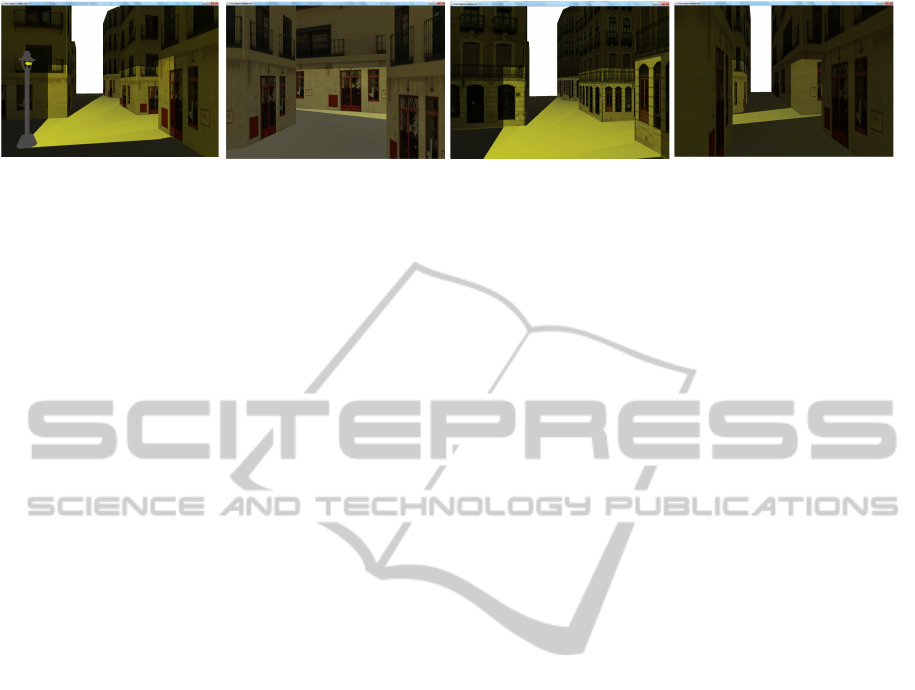
Figure 1: Sample view from a city in which it is only necessary to render a 0.1% of the total geometry.

detail the related previous work. Next, in Section 3 we

deﬁne the polar diagram and its angular characteris-

tics for visibility and shadow determination. Follow-

ing, in Section 4 we detail our approach to be applied

in 2.5D urban scenes. Finally, Section 5 presents our

results and, Section 6 the main conclusions and the

future work.

2 PREVIOUS WORK

Virtual cities have a huge amount of applications such

as trafﬁc simulation, visual impact analysis of ar-

chitectural projects or computer games (Wonka and

Schmalstieg, 1999). In recent years there is a grow-

ing interest in working with virtual cities. Despite

real-time visualization of these environments is a very

challenging problem (Cignoni et al., 2007), there is no

speciﬁc bibliography for realistic rendering of large

cities considering the shadows that buildings cast

(Dorsey and Rushmeier, 2008).

In the literature we can ﬁnd a number of al-

gorithms for massively rendering cities such as the

blockmaps (Di Benedetto et al., 2009) or the texture-

atlas tree (Buchholz and Dollner, 2005). These ap-

proaches usually adapt traditional acceleration strate-

gies (such as level of detail, image-based render-

ing and visibility culling techniques) to the particular

properties of city models: 2.5D overall shape, plane-

dominant geometry, regular structure, dense occlu-

sion, large texture datasets (Argudo et al., 2012) or

geometry simpliﬁcation (Germs and Jansen, 2001).

As stated in (Revanth and Narayanan, 2012),

culling approaches avoid rendering the geometry that

is ultimately not visible, which is especially use-

ful in web-client systems. Occlusion culling tech-

niques perform particularly well in urban environ-

ments (Wonka et al., 2001), in which buildings are

normally big occluders (Koldas et al., 2007). Our pro-

posed method ﬁrstly makes a drastic geometry reduc-

tion using a novel occlusion culling method. Thanks

to this approach, the data that should be processed

are reduced and the GPU is released of rendering big

scenes. The method is based on the polar diagram

(Grima et al., 2006), which performs a plane subdi-

vision on the city map. A similar approach used for

web-based city walks in (Zara, 2006) also generates

a sector division of a virtual city. However, the main

drawback of this proposal is that the division must be

added to the system manually.

Besides visibility culling techniques, another

common strategy to reduce the size of the urban scene

is modeling the buildings as 2.5D models (Bittner

et al., 2005; Cohen-Or et al., 1998). Thus, the prism-

shaped elements can be efﬁciently processed thanks

to this simpliﬁcation process without losing realism

in the ﬁnal scene.

To the best of our knowledge, classical real-time

shadow approaches such as shadow maps or shadow

volumes (Eisemann et al., 2011), are not focused

on very large urban environments, and can be over-

whelmed by the large amount of geometry to be pro-

cessed. As a consequence, this kind of solutions can

be useful in a second step to deal with the reduced

scene (the visible portion from the pedestrian point

of view). There are some strategies to minimize the

impact of the excess of the geometry, like BSP, oc-

tree, etc. For instance, (Chin and Feiner, 1989) pre-

sented the ﬁrst BSP solution related with the compu-

tation of shadows. They proposed the shadow volume

BSP tree where each node is related with a shadow

along a given plane. Each light source requires its

corresponding SVBSP tree. For each tree, the number

of nodes are minimized by grouping shadow areas of

different polygons.

3 THE POLAR DIAGRAM

Visibility resolution is invaluable for the efﬁcient de-

velopment of shadow algorithms under the assump-

tion that only the visible portion of scene must be

rendered. The polar diagram solves visibility for 2D

and 2.5D scenes as described in (Ortega and Robles-

Ortega, 2013) for the general case, and in (Robles-

Ortega et al., 2009) for urban scenes.

In this paper we demonstrate that the polar dia-

gram can also be used to compute shadows using the

same preprocessing. In summary, in a ﬁrst phase of

GRAPP2014-InternationalConferenceonComputerGraphicsTheoryandApplications

the process the polar diagram determines the section

of visible scene from the viewpoint. Afterwards, the

same tessellation determines which portions of this

visible scene are illuminated or in shadow. In this

second phase each light source is in fact used as view-

point to solve the same visibility problem. Visible ar-

eas coincide with the lighted scene when the view-

point is replaced by light sources. Boundaries delim-

iting the illuminated areas and those that remain in

darkness are also determined with complete accuracy

and efﬁciency. The ﬁrst phase for visibility determi-

nation is fully detailed in (Ortega and Robles-Ortega,

2013). This method works with the simple 2D ge-

ometry of the building footprints, but considering the

height of the buildings. It follows a ray-shooting pro-

cess managing tangent lines to this two-dimensional

objects. Tangent lines or bitangent lines are also re-

ferred in the literature to get the visibility complex

of n convex objects in the plane (Pocchiola and Veg-

ter, 1993). The visibility complex has also been used

for radiosity computation in 2D environments (Du-

rand et al., 1996). In this paper we focus on shadows

calculation once the polar diagram has found the ex-

act portion of visible scene.

The polar diagram associated to the scene E,

P (E), can be deﬁned in similar terms to the Voronoi

diagram (Okabe et al., 1992). This tessellation ﬁnds

the nearest site to a given point position in logarith-

mic time by locating this point in a Voronoi region.

The polar diagram follows the same principle: (1) any

point position p is located in the polar region of object

, p ∈ P

) in logarithmic time , (2) and a winged-

edge data structure speeds up ray-shooting algorithms

thanks to the topological relations.

While the Voronoi diagram obtains the nearest site

to a given point (Euclidean distance criterion), the po-

lar diagram ﬁnds the nearest angular site (or polygo-

nal object). That is, it uses the minimum angle as

criterion of construction, which beneﬁts the search of

angularly close objects. The use of polar diagrams

has several advantages such as being precomputed in

optimal time, Θ(nlogn), and also that conservativity

is ensured, which means that no visible objects are

missed.

The major drawback is that no speciﬁc methods

have been developed for 3D scenes. However, the ex-

tension to 2.5D scenes is straightforward. Although

visibility determination is considered a complex prob-

lem in 3D scenes, urban environments have certain

characteristics that make visibility to be addressable

using polar diagrams. Buildings can be considered

large occluders that are usually represented by prism-

shaped objects, the so-called 2.5D models (Cohen-Or

et al., 2003).

(a) Top view scene (b) P

(E)

Figure 2: Visibility and illumination relationship.

Figure 2.a) represents the top view of a prism-

shaped scene. The leftmost picture shows the por-

tion of scene directly illuminated by a light source

or directly visible by an observer. These problems

can be directly solved in linear time by performing a

clockwise and counterclockwise scanning from p as

depicted in Figure 2.b). However, this calculation is

expensive in time if the scene is very large or the ob-

server moves. In this picture p is located in the polar

region of object B. By deﬁnition of polar diagram, if

p ∈ P

(B), object B is the ﬁrst visible object from p

when performingan angular scanning from angle zero

in counterclockwise direction, and therefore, B is vis-

ible from p. If this polar diagram works efﬁciently in

the angular range [0,π/2], the total angular spectrum

[0,2π] can be covered using four polar diagrams, each

of them working in a similar way for each of the four

quadrants of the coordinate plane as described in (Or-

tega and Robles-Ortega, 2013).

Although angular proximity does not involve vis-

ibility, it identiﬁes which are the candidates that must

be checked. The resulting illuminated scene is iden-

tiﬁed by means of a ray-casting process from point

p using the plane partition obtained by the polar dia-

gram.

3.1 The Ray-casting Process

Visibility or illumination can be solved by means

of a ray-casting process from the viewpoint or light

source. Any ray shot r(t) from p in the angular range

[0,π/2], representing a light beam, can use the P (E)

polar diagram to determine efﬁciently its trajectory

using the topological data structure associated to po-

lar diagrams. If r(t) intersects with object o

, then

is visible from p. If a single ray can determine a

visible object in a speciﬁc direction, then a fan of se-

lected rays may determine the visible portion of the

scene from p in an angular range. The view frustum

is deﬁned by the angular sector [r

], being r

the

ray deﬁning the left side and r

the right one. If the

view frustum does not match with a quadrant, which

is the usual, two or more polar diagrams will be used

ANovelRay-shootingMethodtoRenderNightUrbanScenes-AMethodbasedonPolarDiagrams

as described next (Ortega and Robles-Ortega, 2013):

1. Divide [~r

, ~r

] into the sub-intervals correspond-

ing to each quadrant involved.

2. For each sub-interval [~r

, ~r

] ⊆ [~r

, ~r

]

(a) Determine the polar diagram P (E) for this sub-

interval.

(b) Locate p in the polar region of object o

, p ∈

, r

, ...,r

} being for simplicity

= r

(t), j ∈ [l,1,2,...,r] a ray starting

from the light source position p.

(d) For each ray r

compute a collision detection.

Of all the above steps, which deserve explanation

are the collision detection process and the selection of

rays. The collision detection (Step 2.(d)) is discussed

in (Ortega and Feito, 2005). This process provides,

the object o

intersecting with r(t) (if any). Then, o

is visible from p and depending on the distance, o

directly illuminated. The algorithm describes the tra-

jectory of r(t) through adjacent polar regions until an

intersection is computed or the ray leaves the scene.

The ray shooting process requires O(N) time for

guiding the ray r(t) across the N regions of the scene.

However, the worst case is very rare in dense scenes in

which the ray is likely to collide with nearby objects.

Algorithm 1: Fan of tangent rays R

Input:

• The scene E = {o

,...,o

}

• The light source position p

Output: The fan of tangent rays R

= {r

, r

, ...,r

}

BEGIN

1. Let V the set of visible objects from p, V =

2. Let T =

0 a data structure of rays angularly sorted from

left to right

3. Insert r

and r

into T

4. While T is not empty

(a) Get and remove the ﬁrst element r

from T

(b) Insert r

into R

and detect the collision with object objInt

(d) Determine [r

j+1

] the consecutive rays in R

such

that r

∈ [r

j+1

]

(e) If objInt 6= Null AND objInt /∈ V AND [r

j+1

] is

not a closed range

i. Insert objInt into V

ii. Insert in T the left and right tangent to object o

5. return R

angularly sorted

END

Next we deﬁne the tangent ray and fan of tangent

rays concepts:

Deﬁnition 1. The tangent ray: r

= {p, ptTg,

objTg, ptInt, ob jInt} represents the set of attributes

associated to the ray r

, being p the origin of the ray

(viewpoint), objInt ∈ E is the object collided by r

the point ptInt, ob jTg ∈ E is the object such that r

tangent to ob jTg and ptTg is the tangent point of r

objTg. We denote R

= {r

, r

, ..., r

} as the the

fan of tangent rays with origin in p, angularly sorted

and using a single polar diagram P (E).

All these tangent rays r

form the corresponding

fan of tangent rays R

which ﬁnds exact visibility.

The advantages of tangent lines are that the set R

as reduced as possible (only O(2k) rays for k visible

objects). In addition light sources also follow tangent

lines direction, which makes our method especially

suitable for illumination purposes.

The ray-casting process described in Algorithm 1

generates a fan of rays angularly sorted from p. Each

ray launched may detect a new visible object o

which

is inserted in the set V of visible objects. Then the left

and right tangent lines to o

are inserted in the set T

of rays to be processed in the same way. The result is

a fan of tangent rays described above deﬁning the ex-

act illuminated areas of the scene (see Deﬁnition 1).

Each tangent ray is determined by the origin and end

point of r

, the visible object objInt and its intersect-

ing point ptInt, as well as the information about the

tangent object ob jTg, if any, and the tangent point

ptTg.

The algorithm follows inserting the two rays

deﬁning the view-frustum r

and r

in T (Step 3). r

is the ﬁrst ray angularly sorted and the ﬁrst one that

is shot. Whenever a launched ray r

intersects with

an object objInt, its left and right tangent rays are in-

serted in T to be processed later, but only if this new

ray satisﬁes the following conditions:

• it is in the range [~r

, ~r

]

• it does not collide with any object already inserted

in V (if is not already visible)

• it is not within a closed range in R

Two neighbors rays r

and r

j+1

, r

j+1

∈ R

pro-

vide a closed range if the angular sector [r

j+1

] only

contains one object. Otherwise, the new tangent ray is

inserted in T waiting to be processed in order to ﬁnd

new visible objects. When a tangent ray lies into a

closed range or it intersects with a visible object, no

additional rays are necessary to ﬁnd new objects. Oth-

erwise, r

and r

j+1

may contain more than one object

and the algorithm must shot new tangents rays and

identify which objects may be placed within [r

j+1

]

(Step 4(d)).

GRAPP2014-InternationalConferenceonComputerGraphicsTheoryandApplications

P P

Figure 3: Fan of rays from point p.

The example of Figure 3 depicts the resulting fan

of rays determining visible objects from point p after

applying Algorithm 1. Initially, T = {r

} (Step 3),

the ﬁrst ray shot is r

which collides with object o

(Step 3(c)). The right tangent to o

, the ray r

is shot

(the left one is out of range and is not considered)

reaching o

. At this point V = {o

} contains two

visible objects. The new rays shot are r

and r

, the

left and right tangent rays to o

respectively. Among

, r

and r

the visible range is closed now because

only one object is within each pair of these rays. The

process follows when T becomes empty andV ﬁnally

contains the visible set of objects.

The topological data structure of polar diagrams

guides efﬁciently each tangent ray across the scene,

and also ensures to get exactly the illuminated area.

The rest of the scene remains in shadow.

Algorithm 1 shoots O(k) rays to determine k vis-

ible objects, which is optimal. As each ray can cross

O(N) polar regions to achieve a visible object, in the

worst case the fan of rays needs O(kn) time for ﬁnding

the visibility set. However, the illumination process is

more efﬁcient than visibility since objects cannot be

illuminated beyond a speciﬁc distance. Then, illumi-

nation can be solved in O(k), being k the number of

illuminated objects.

4 DETERMINING THE

SHADOWED AND

ILLUMINATED AREAS

The fan of tangent rays determines the visible objects

from the light source position, and also the frontier

between their shadowed and lit areas, as described be-

low.

(a) Illumination from a

light source.

Secondary

(b) Umbra points gener-

ated by two tangent rays

Figure 4: Classiﬁcation of hit points.

4.1 Algorithm Details

Once the fan of tangent rays has been computed, the

following step is the classiﬁcation of the hit points

(Deﬁnition 2) as primary or secondary points. A hit

point is considered as primary if a tangent ray directly

intersects with any other object before touching the

tangent object (as points v1 and v2 in Figure 4(a)).

On the contrary, if the ray hits ﬁrst the tangent object

before intersecting with any other in the scene, then

this hit point is classiﬁed as secondary. These points

are the frontier between shadowedand illuminated ar-

eas as depicted in the example of Figure 4(b). In this

case, rays r1 and r2 touch object A before intersecting

with B. Therefore, A casts a shadow on B, and points

v1 and v2 should be considered as secondary points.

The attributes of a hit point are formally described in

Deﬁnition 2.

Deﬁnition 2. The hit point: vp =

{p,obj,illuminated} represents the 2D intersecting

point p between a tangent ray and the polygon obj;

illuminated is an attribute which classiﬁes the point

as primary when true or secondary otherwise.

The process to determine the set of hit points from

the fan of tangent rays is described in Algorithm 2.

Each tangent ray is likely to intersect with any build-

ing in a hit point. These points are highly relevant in

our method because they deﬁne the border between

light and shadowy areas. Then, the method evaluates

these hit points as primary or secondary. Speciﬁcally,

there are four possible cases for each ray which are

next described.

The ﬁrst case (step 2a in Algorithm 2) considers

the non-tangent rays r

and r

, deﬁning the angular

range (see Algorithm 1). These rays are the only ones

that are non-tangent to any object. They may not in-

tersect with any polygon, and then the algorithm fol-

lows with other rays. Otherwise, if the intersection is

computed, the hit point is considered as primary,since

there is no other object involved. This is the step 2b

in the algorithm, illustrated in Figure 5.

The next case is a non-intersecting tangent ray as

ANovelRay-shootingMethodtoRenderNightUrbanScenes-AMethodbasedonPolarDiagrams

Algorithm 2: Obtain and classify the hit points.

Input:

• The fan of tangent rays R

= {r

, r

, ...,r

}

• The light source position p

Output: The set of hit points S

= {vp

, vp

, ...,vp

vpn

}

BEGIN

1. S

= 0

2. For each ray r

in R

(a) If r

.ptTg is null AND r

.ptInt is null Then continue

(b) If r

.ptTg=Null AND r

.ptInt 6= Null Then (Fig. 5)

i. S

+ = HitPoint(r

.ptInt,r

.objInt,true);

.ptTg6=Null AND r

.ptInt=Null Then (Fig. 6)

i. S

+ = HitPoint(r

.ptTg,r

.objTg,true)

(d) If r

.ptTg6=Null AND r

.ptInt6=Null Then

i. If (distance(lp,r

.ptTg) < distance(lp,r

.ptInt))

Then (Fig. 7(a))

A. S

+ = HitPoint(r

.ptTg,r

.objTg,true);

B. S

+ = HitPoint(r

.ptInt,r

.objInt,false);

ii. else (Fig. 7(b))

A. S

+ = HitPoint(r

.ptInt,r

.objInt,true);

END

depicted in Figure 6 (step 2c). The hit point r

.ptTg is

considered as primary because there are not obstacles

between object A and the light source.

There are two possible situations when a tangent

ray intersects with any object (step 2d): the tangent

object is in front or behind of the hit object. The ﬁrst

case is classiﬁed as primary like Figure 7(a) shows.

In this example, object A is closer than B to the light

source position. Therefore, as A casts a shadow in

object B, ptInt is secondary and ptTg is primary. The

other situation (Figure 7(b)) is the opposite because

objTg, object B in this case, is behind the object A,

which determines that ptInt is primary. In this case,

ptTg should not be considered for classiﬁcation since

it is not directly illuminated from the light source.

An example of the hit points obtained using the

Algorithm 2 in a full scene is shown in Figure 3. As

depicted in the picture, each ray determines one or

two of these intersecting points. For example, ray r

obtains two hit points (the ﬁrst in object 1 and the

second in object 2). Nevertheless, ray r

only in-

cludes one because the tangent point in object 5 is not

reached from the light source.

4.2 Generating the Illuminated Faces of

the Polygons

After classifying the hit points, the next step is deter-

mining if the polygon areas between two consecutive

hit points are illuminated or shadowed (Deﬁnition 3).

(a) r

.ptInt is primary. (b) r

.ptInt is primary.

Figure 5: Examples for case 2b in Algorithm 2.

















(a) Point r

.ptTg is primary.

Figure 6: Example for case 2c in Algorithm 2.

Deﬁnition 3. The polar area: va = {v,illuminated}

represents an interval which delimits the illuminated

area of a polygon, being v = {v

,...,v

} the set of

polygon vertices delimiting the area and illuminated

an attribute that classiﬁes the area as illuminated or

umbra. If illuminated is true, then the area has to be

represented as lit, otherwise, it is shadowed.

The area between two adjacent rays of the fan

of tangent rays are deﬁned as the polar area. Each

of these angular sectors is illuminated or shaded,

whereby each of these areas will be rendered in ac-

cordance with its classiﬁcation: illuminated or umbra.

The polar areas are built using the polygon vertices

and the hit points, according to the process summa-

rized in Algorithm 3. This procedure can be divided

into two main parts: 1) obtaining the points which

compose the area and 2) determining if they are illu-

minated or not.

Each area considered as illuminated or umbra is

delimited by two consecutive hit points (v

and v

i+1

ght

source

ptTg

(Primary)

ptInt

(Secondary)

(a) r

.ptTg is primary

and r

.ptInt is secondary.

ght

source

ptInt

(Primary)

ptTg

(not visible)

(b) r

.ptInt is primary and r

.ptTg

is not needed as it is behind the

building.

Figure 7: Examples for case 2d in Algorithm 2.

GRAPP2014-InternationalConferenceonComputerGraphicsTheoryandApplications

ght

source

Primary

(a) Considering tangent

and non-tangent rays.

(b) Only considering tan-

gent rays.

Figure 8: Examples for case 6 in Algorithm 3.

All polygon vertices between v

and v

i+1

are also con-

sidered for generating the illuminated or umbra geom-

etry in the scene. (Steps 3-5 in the algorithm).

Algorithm 3: Classify the polar areas of a polygon.

Input:

• The set of hit points S

= {vp

, vp

, ..., vp

vpn

} associ-

ated to an object o

• The vertices deﬁning the perimeter of objects O =

, o

, ...,o

}

Output: The set of polar areas of the polygon, S

{vp

, vp

, ...,vp

van

}

BEGIN

For i=1 To vpn-1

1. Let be va a polar area

2. va.v ←

3. va.v+=vp

insert the ﬁrst hit point

4. va.v+=O insert the rest of polygon vertices between vp

and vp

i+1

5. va.v+=vp

i+1

insert the last hit point

6. If (vp

.illuminated AND vp

i+1

.illuminated) Then

va.illuminated =True (Fig. 8)

7. If ( (NOT vp

.illuminated AND vp

i+1

.illuminated) OR

(vp

.illuminated AND NOT vp

i+1

.illuminated) ) Then

(a) va.illuminated =true (Fig. 9)

8. If (NOT vp

.illuminated AND NOT vp

i+1

.illuminated)

Then

(a) If (vp

.obj == vp

i+1

.obj) Then

i. va.illuminated =false (Fig. 10(a))

(b) else

i. va.illuminated =true (Fig. 10(b))

END

Once all the vertices of the polar area have been

inserted, next we determine if this area is shadowed

by analyzing the three possible cases of the vertices v

and v

i+1

1. If both points v

and v

i+1

are primary (Step 6),

then the polar area is considered as illuminated.

In Figure 8 the hit points determine a lit part of

object A.

Figure 9: Examples for case 7 in Algorithm 3.

Secondary

(a) Hit points are sec-

ondary, and the area be-

tween v

and v

is shad-

owed.

Secondary

Light

source

Secondary

(b) Hit points are sec-

ondary, but the marked area

is illuminated

Figure 10: Examples for case 8 in Algorithm 3.

2. If one of the hit point is primary and the other sec-

ondary (Step 7, Figure 9), then the area is illu-

minated since there are no obstacles between the

light source and the object.

3. If both hit points v

and v

i+1

are secondary (Step 8,

Figure 10) then two different cases are found de-

pending on the object associated to the hit points:

(a) If both hit points are generated from the same

polygon, then the area is umbra. Figure 10(a)

shows an example, v1 and v2 are tangent points

of object A, which partially occludes the light

toward polygon B.

(b) If the hit points are tangent to different objects,

as in Figure 10(b), then these points determine

an illuminated area, since there are no obstacles

between the light source and the object.

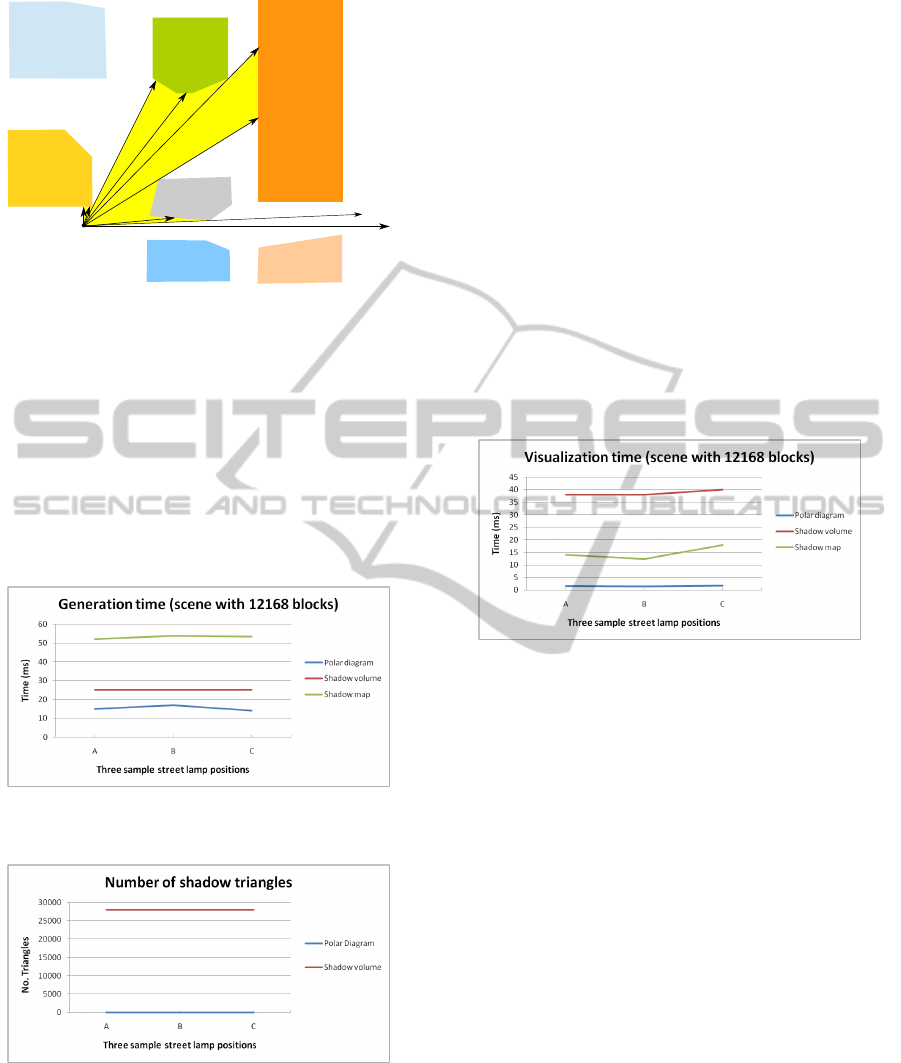
Figure 11 shows the polar areas of the scene of

Figure 3. According to Algorithm 3, two consecutive

primary points determine an illuminated area, as in

the case of object 1. An example of two consecutive

secondary points can be seen for object 5, however

the area between them is illuminated because these

two points have been generated from different objects

(step 8b in the algorithm).

Finally, the polar areas are used to create the 3D

model of both ﬂoor and building faces. In the ﬁrst

case, the illuminated parts of the ﬂoor are generated

using the triangles shown in Figure 11. These trian-

gles are built using the origin and endpoint of each

polar area and the light source position. On the other

hand, building faces are created by an extrusion pro-

ANovelRay-shootingMethodtoRenderNightUrbanScenes-AMethodbasedonPolarDiagrams

Figure 11: Determining and classifying the polar areas.

cess which uses the vertices of the polar areas.

5 RESULTS AND DISCUSSION

This section presents the tests carried out using an

Intel

Core

2 Quad CPU Q2800 2.33GHz to eval-

uate the performance and accuracy of our method.

Next we describe them in detail.

Figure 12: Generation time of three sample street lamp po-

sitions.

Figure 13: Number of triangles of three sample street lamp

positions.

The former test compares our approach with an-

other classical shadow techniques like shadow maps

and shadow volumes with regard to performance.

Speciﬁcally, two different urban scenes composed

of 1183 and 12168 blocks of buildings (7.000 and

70.000 triangles respectively) have been used. For

each scene, three representative street lamp positions

(A, B and C) have been selected in different areas of

the city in order to study the number of shadow trian-

gles, and the generation and visualization time.

Table 1 summarizes the results for the polar di-

agram (top), shadow volume (medium), and shadow

map (bottom). In the case of the polar diagram, the

shadow computation time is divided into the time re-

quired to ﬁnd the lit set of blocks and the ground

surface. Despite this process is straightforward for

shadow maps and shadow volumes, our method is

faster (see Figure 12). The construction time and

the visibility determination for polar diagrams can be

considered as a pre-processing phase because build-

ings do not change and street lamps do not move dur-

ing the navigation process. Therefore, these times

should not be considered in the performance study.

Figure 14: Visualization time of three sample street lamp

positions.

Another important feature associated to our ray-

casting method is its accuracy in 2.5D scenes, since it

ﬁnds the exact set of directly illuminated primitives.

As a result, the shadow geometry to be rendered in the

scene is considerably reduced in comparison with the

shadow volume technique which requires the genera-

tion of a signiﬁcant amount of extra geometry (Eise-

mann et al., 2011). In our example, thousands of

triangles are needed to represent the shadow volume

while the polar diagram only uses dozens of polygons

(see Figure 13).

Besides generation time and geometry, another

important feature in performance is the visualization

time. As shown in Table 1 and Figure 14, the ren-

dering time is also more reduced for our method (on

average of about 20 times). This is a direct conse-

quence of the shadow geometry reduction since the

ﬁnal scene to be rendered is smaller than for the clas-

sical approaches.

In view of the results of this test, we can conclude

that our method obtains a good performance in 2.5D

scenes with regard to generation, rendering times, and

geometry load. This issue is specially useful for web-

based systems and low-capacity devices.

GRAPP2014-InternationalConferenceonComputerGraphicsTheoryandApplications

Table 1: Performance of polar diagrams, Shadow Map and Shadow Volume. Scene A(7000 triangles), Scene B(70000 trian-

gles).

Scene A (1183 blocks) Scene B (12168 blocks)

Street lamp positions (A,B,C)

A B C

Polar Diagram

Construction time (ms) 437 1940

No. visible buildings

1 2 2 4 2 3

Time to determine visibility (ms)

30 30 10 42 29 30

Ground shadows (No. triangles)

3 4 7 5 4 11

Ground shadows (cpu time ms)

2 1 2 13 14 13

Block shadows (No. triangles)

9 18 18 8 6 6

Block shadows (cpu time ms)

1 1 1 2 3 1

Visualization (time ms)

1 1 1 1.5 1.33 1.67

Shadow Volume

No. vertices

9464 9464 9464 56000 56000 56000

No. Quads

2366 2366 2366 14000 14000 14000

Shadow generation (No. triangles)

4732 4732 4732 28000 28000 28000

Shadow generation (cpu time ms)

10 10 9.5 25 25 25

Visualization (time ms)

6 8 7 38 38 40

Shadow Map

Shadow generation (cpu time ms)

14 14 13 52 54 53.5

Visualization (time ms)

6 8 7 14 12.3 18

The main purpose of the latter test is studying the

behaviour of our method during a free walkthrough

navigation (see four sample screenshots of this pro-

cess in Figure 1). Speciﬁcally, the navigation process

has been evaluated at ﬁve positions as reﬂected in Ta-

ble 2. These results show how the number of trian-

gles has considerably been reduced, the system man-

ages less than 100 triangles instead of the 70.000 from

the original scene. Therefore we obtain an important

reduction representing the 0,14% of the global scene

geometry.

With regards to graphical results, Figure 15 shows

the same urban scene with different kind of illumina-

tions. The ﬁrst image (Figure 15(a)) depicts the scene

after disabling all sources of light. The second image

(Figure 15(b)) considers the same night scene with

local illumination from a single light source with-

out shadows. Finally, the last image shows the night

scene with local illumination and the shadows gener-

ated by our method.

Another important advantage of our method is the

reduced amount of memory needed to store the polar

diagram structure. As Table 3 shows, the four po-

lar diagrams only take up 175.125 bytes. This value

is signiﬁcantly low considering the high capacity of

the current computers, and the beneﬁts obtained by

our approach described above. The table details the

memory requirements for each one of the polar dia-

gram components: polar axis (border lines between

polar regions), polar regions, polygons of the scene,

Table 2: Results for navigation using Polar Diagrams.

Position A B C D E

No. visible buildings 5 2 3 2 2

No. Building triangles 60 24 42 18 36

No. Ground triangles 30 12 21 9 18

Generation time (ms) 14 9 9 9 9

Visualization time (ms) 1 1 1 1 1

Table 3: Memory requirements (in bytes) for polar dia-

grams.

East+ East- West- West+ Total

Polar

axis

7,031 6,563 7,031 6,563 27,188

Polar

regions

21,5 19,938 20,75 21,063 83,25

Polygons 11,969 11,969 11,969 11,969 47,875

Rest of

ﬁelds

4,063 4,063 4,344 4,344 16,813

Total 44,563 42,531 44,094 43,938 175,125

and the rest of ﬁelds of the data structure.

6 CONCLUSIONS AND FUTURE

WORK

In this paper we have proposed a novel real-time

method based on polar diagrams to navigate through

night large virtual cities. The main strength of this

ANovelRay-shootingMethodtoRenderNightUrbanScenes-AMethodbasedonPolarDiagrams

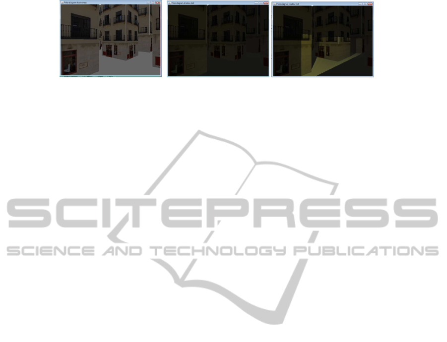
(a) No lighted scene (b) Night scene. Local illu-

mination without shadows

mination and shadows gen-

erated using our method

Figure 15: Visual results.

method is the minimization of the geometry to be ren-

dered for a givenposition, independentlyof the size of

the scene. This feature makes this ray-casting method

suitable to be used for lighting large urban environ-

ments in web-based systems or low-capacity devices.

In view of the results, for 2.5D urban scenes, our visu-

alization times have outperformed those obtained by

classical methods like shadow maps and shadow vol-

umes. Moreover, as our algorithm is independent of

the screen resolution it is guaranteed the maximum

quality with different kind of devices and without any

additional geometry processing.

For future work we also consider to implement the

proposed algorithms in the GPU by using OpenCL

or WebCL. In our opinion we would take advantage

of parallelizing the ray-casting process as well as the

polar diagram construction. Furthermore, we want to

extend our method to deal with mobile light sources

since the topological relationships associated to polar

diagrams enable the extension of this problem, as well

as for navigation (Robles-Ortega et al., 2009). We

think it is possible to obtain good results with a low

extra cost.

As this paper is focused on urban scenes, the

buildings remain static during the whole process.

However, we plan to study the cost of a dynamic up-

dating of the polar diagram. This scenario could be

useful in other 2.5 environments.

In addition, as it has been shown, once the polar

diagram has been generated, the computation of the il-

lumination region from a new light source is achieved

in real time. This outcome evinces the possibility of

extending, in a future work, the current proposal to

indirect illumination based on virtual point lights, for

instance.

Another possible extension is the use of area light

sources in order to generate soft shadows. The polar

diagram give us a good understanding of the neigh-

borhood and, intrinsically, it is not limited to point

light sources. In that case, the portion of the area light

source, visible from a given position, should be some-

how determined.

ACKNOWLEDGEMENTS

This work has been partially granted by the Con-

serjer´ıa de Innovaci´on, Ciencia y Empresa of the

Junta de Andaluc´ıa, under the research project

P07-TIC-02773

REFERENCES

Argudo, O., And´ujar, C., and Patow, G. (2012). Interactive

rendering of urban models with global illumination. In

Computer Graphics International, Bournemouth Uni-

versity, United Kingdom.

Bittner, J., Wonka, P., and Wimmer, M. (2005). Fast ex-

act from-region visibility in urban scenes. In Bala,

K. and Dutr, P., editors, Rendering Techniques 2005

(Proceedings Eurographics Symposium on Render-

ing), pages 223–230. Eurographics, Eurographics As-

sociation.

Buchholz, H. and Dollner, J. (2005). View-dependent ren-

dering of multiresolution texture-atlases. In Visualiza-

tion, 2005. VIS 05. IEEE, pages 215–222.

Chin, N. and Feiner, S. (1989). Near real-time shadow gen-

eration using bsp trees. ACM SIGGRAPH Computer

Graphics, 23(3):99–106.

Cignoni, P., Di Benedetto, M., Ganovelli, F., Gobbetti, E.,

Marton, F., and Scopigno, R. (2007). Ray-casted

blockmaps for large urban models visualization. Com-

puter Graphics Forum, 26(3):405–413.

Cohen-Or, D., Chrysanthou, Y., Silva, C., and Durand, F.

(2003). A survey of visibility for walkthrough appli-

cations. Visualization and Computer Graphics, IEEE

Transactions on, 9(3):412 – 431.

Cohen-Or, D., Fibich, G., Halperin, D., and Zadicario, E.

(1998). Conservative visibility and strong occlusion

for viewpace partitioning of densely occluded scenes.

In EUROGRAPHICS’98, volume 17, pages 243–253.

Di Benedetto, M., Cignoni, P., Ganovelli, F., Gobbetti, E.,

Marton, F., and Scopigno, R. (2009). Interactive re-

mote exploration of massive cityscapes. In The 10th

International Symposium on Virtual Reality, Archae-

ology and Cultural Heritage VAST (2009), pages 9–

16. Eurographics.

GRAPP2014-InternationalConferenceonComputerGraphicsTheoryandApplications

Dorsey, J. and Rushmeier, H. (2008). Light and materials

in virtual cities. In ACM SIGGRAPH 2008 classes,

SIGGRAPH ’08, pages 8:1–8:4, New York, NY, USA.

ACM.

Durand, F., Orti, R., Rivi`ere, S., and Puech, C. (1996).

Radiosity in ﬂatland made visibly simple: using the

visibility complex for lighting simulation of dynamic

scenes in ﬂatland. In Proceedings of the twelfth an-

nual symposium on Computational geometry, SCG

’96, pages 511–512, New York, NY, USA. ACM.

Eisemann, E., Schwarz, M., Assarsson, U., and Wimmer,

M. (2011). Real Time Shadows. A K Peters/CRC

Press.

Germs, R. and Jansen, F. W. (2001). Geometric simpliﬁca-

tion for efﬁcient occlusion culling in urban scenes. In

Proc. of WSCG 2001, pages 291–298.

Grima, C. I., Marquez, A., and Ortega, L. (2006). A new 2d

tessellation for angle problems: The polar diagram.

Computational Geometry. Theory and Applications,

34(2):58 – 74.

Koldas, G., Isler, V., and Lau, R. W. H. (2007). Six degrees

of freedom incremental occlusion horizon culling

method for urban environments. In ADVANCES IN

VISUAL COMPUTING, PT I, volume 4841 of Lecture

Notes in Computer Science, pages 792–803.

Musialski, P., Wonka, P., Aliaga, D. G., Wimmer, M., van

Gool, L., and Purgathofer, W. (2013). A Survey of

Urban Reconstruction. Computer Graphics Forum,

Early View.

Okabe, A., Boots, B., and Sugihara, K. (1992). Spatial Tes-

sellations: Concepts and Applications of Voronoi Di-

agrams. John Wiley and Sons.

Ortega, L. and Feito, F. (2005). Collision detection using

polar diagrams. Computer & Graphics, 29(5):726–

737.

Ortega, L. and Robles-Ortega, M. D. (2013). Applied math-

ematics & information sciences. ACM Trans. Graph.,

pages 1651–1669.

Pocchiola, M. and Vegter, G. (1993). The visibility com-

plex. In Proceedings of the ninth annual symposium

on Computational geometry, SCG ’93, pages 328–

337, New York, NY, USA. ACM.

Revanth, N. R. and Narayanan, P. J. (2012). Dis-

tributed massive model rendering. In Proceedings

of the Eighth Indian Conference on Computer Vision,

Graphics and Image Processing, ICVGIP ’12, pages

42:1–42:8. ACM.

Robles-Ortega, M., Ortega, L., Coelho, A., Feito, F., and

de Sousa, A. (2013). Automatic street surface model-

ing for web-based urban information systems. Journal

of Urban Planning and Development, 139(1):40–48.

Robles-Ortega, M. D., Ortega, L., and Feito, F. (2009). An

exact occlusion culling method for navigation in vir-

tual architectural environments. In Proceedings of the

IV Iberoamerican Symposium in Computer Graphics,

pages 23–32.

Wonka, P. and Schmalstieg, D. (1999). Occluder shadows

for fast walkthroughs of urban environments. Com-

puter Graphics Forum, 18(3):51–60.

Wonka, P., Wimmer, M., and Sillion, F. (2001). Instant visi-

bility. Computer Graphics Forum, 20(3):C411+. 22nd

Annual Conference of the European-Association-for-

Computer-Graphis, MANCHESTER, ENGLAND,

SEP 04-07, 2001.

Zara, J. (2006). Web-based historical city walks: advances

and bottlenecks. Presence: Teleoper. Virtual Environ.,

15(3):262–277.

ANovelRay-shootingMethodtoRenderNightUrbanScenes-AMethodbasedonPolarDiagrams