
Speeding Up Object Detection
Fast Resizing in the Integral Image Domain
Michael Gschwandtner, Andreas Uhl and Andreas Unterweger
Department of Computer Sciences, University of Salzburg, Jakob-Haringer-Straße 2, Salzburg, Austria
Keywords:
Integral Image, Resizing, Object Detection, Performance.
Abstract:
In this paper, we present an approach to resize integral images directly in the integral image domain. For the
special case of resizing by a power of two, we propose a highly parallelizable variant of our approach, which
is identical to bilinear resizing in the image domain in terms of results, but requires fewer operations per pixel.
Furthermore, we modify a parallelized state-of-the-art object detection algorithm which makes use of integral
images on multiple scales so that it uses our approach and compare it to the unmodified implementation.
We demonstrate that our modification allows for an average speedup of 6.38% on a dual-core processor with
hyper-threading and 12.6% on a 64-core multi-processor system, respectively, without impacting the overall
detection performance. Moreover, we show that these results can be extended to a whole class of object
detection algorithms.
1 INTRODUCTION
Integral images, initially developed under the name
”summed-area tables” (Crow, 1984), have regained
a lot of attention since Viola and Jones proposed an
object detection framework (Viola and Jones, 2001)
which makes heavy use of them. Popular implemen-
tations of this framework, such as the OpenCV li-
brary (Willow Garage, 2012), perform object detec-
tion on multiple scales, i.e., they resize the original
image multiple times and run the detection algorithm
on each resized image, also referred to as scale. Al-
though the object detection is relatively fast due to the
use of integral images, the need to recompute the in-
tegral image for each scale impacts the performance
significantly. Therefore, in this paper, we propose a
new algorithm which allows resizing the integral im-
ages themselves, i.e., in the integral image domain in-
stead of the image domain, omitting the need to re-
compute the integral image for each scale.
Despite efforts to speed up the computation of
integral images in general (Hensley et al., 2005) as
well as on different architectures like GPUs (Bilgic
et al., 2010), literature on integral images is sparse.
While Crow (Crow, 1984) initially described how to
perform simple operations, like, e.g., blurring, in the
integral image domain, Heckbert (Heckbert, 1986)
generalized the underlying theory, thereby extend-
ing its scope to arbitrary filters with polynomial ker-
nels. Hussein (Hussein et al., 2008) improved and
extended Heckbert’s work by enabling non-uniform
filtering. Although both frameworks, Heckbert’s and
Hussein’s, allow to perform resizing operations, they
take input from the integral image domain and pro-
duce output in the image domain. In contrast, our ap-
proach performs all operations directly in the integral
image domain, hereby omitting the need to recompute
the integral image after resizing.
Although algorithms performing operations di-
rectly in the integral image domain have been pro-
posed (e.g., (Yu et al., 2010) for histogram threshold-
ing), none of them changes the size of the integral
image itself, as opposed to the algorithm we propose.
As performing operations on multiple scales in the in-
tegral image domain is part of several state-of-the-art
algorithms, such as SURF (Bay et al., 2008), local
binary patterns (LBP) (Ahonen et al., 2004) and Vi-
ola’s and Jones’ framework for object detection as ex-
plained above, our main contribution of resizing in the
integral image domain inherently allows speeding up
algorithms relying on the computation of integral im-
ages on multiple scales. Note that, although some al-
gorithms allow scaling up the features instead of scal-
ing down the integral images, a significant number of
implementations (Willow Garage, 2012) recompute
the integral images and thus profit from our contri-
bution.
This paper is structured as follows: In section 2,
64
Gschwandtner M., Uhl A. and Unterweger A..
Speeding Up Object Detection - Fast Resizing in the Integral Image Domain.
DOI: 10.5220/0004678000640072
In Proceedings of the 9th International Conference on Computer Vision Theory and Applications (VISAPP-2014), pages 64-72
ISBN: 978-989-758-003-1
Copyright
c
2014 SCITEPRESS (Science and Technology Publications, Lda.)

we propose an algorithm for resizing in the integral
image domain without distortions by imposing cer-
tain restrictions on the resizing factor. In section 3,
we extend this algorithm to support arbitrary resiz-
ing factors, albeit at the cost of negligible distortions.
After evaluating our algorithm in section 4 in terms
of performance, quality and parallelizability, we con-
clude our paper in section 5.
2 EXACT RESIZING
In the following sections we describe how a given in-
tegral image can be resized. We distinguish between
exact and approximate resizing, where exact means
that each pixel of the resized integral image is iden-
tical to the corresponding pixel of an integral image
which is calculated from a bilinearly resized version
of the original image, the resizing process of which
has been performed in the image domain.
2.1 Integral Images
An integral image II of a given image I represents the
sum of all its pixels from the top-left corner to ev-
ery pixel, excluding the column and row of the pixel
(note that some definitions include the pixel’s column
and row, requiring corresponding changes in the sub-
sequent formulas). Hence, it is calculated as (Willow
Garage, 2012)
II(x, y) =
x−1
∑
x
0
=0
y−1
∑
y
0
=0
I(x
0
, y
0
) (1)
This allows calculating the sum S of all pixels within
a rectangular area R in constant time (Crow, 1984) as
S
R
= II(x
r
, y
b
)−II(x
l
, y
b
)−II(x
r
, y
t
)+II(x
l
, y
t
) (2)
where x
l
, x
r
, y
t
and y
b
are R’s left, right, top and bot-
tom coordinates, respectively, as depicted in figure 1.
Note that, in order to reconstruct single pixels from
the integral image (see next section for details), the
integral image’s dimensions are (w+ 1) · (h +1) if the
original image’s dimensions are w · h.
2.2 Na
¨
ıve Resizing
Resizing algorithms usally perform operations in the
image domain, i.e., on the image’s pixels. As be-
comes clear from equation (2), it is possible to extract
every single pixel as a rectangle of width and height
one of the original image I from its integral image II:
I(x, y) =II(x, y) + II(x + 1, y + 1)−
II(x, y + 1) − II(x + 1, y)
(3)
Figure 1: Use of an integral image for summing all pixels
within a rectangular area R constrained by its coordinates
x
l
, x
r
, y
t
and y
b
. Adopted from (Crow, 1984).
Therefore, it is theoretically possible to implement
any image-domain-based resizing filter in the integral
image domain by filtering using on-the-fly extraction
of the original image’s pixels and subsequent calcula-
tion of the resized image’s integral image.
However, this is computationally more expensive
as accessing each pixel requires four operations in the
integral image domain as opposed to one in the image
domain. Furthermore, it is necessary to access loca-
tions in the integral image which are one row apart
in order to derive a single pixel of the original image.
This may cause a higher number of the CPU’s cache
lines to be occupied, if the integral image is stored
sequentially in memory.
2.3 Resizing by a Power of Two
In the following section we propose a resizing algo-
rithm for integral images which eliminates the need
to extract the original image’s pixels from the integral
image in a computationally expensive way. However,
for the algorithm to work exactly, the resizing factor
needs to be a power of two. Note that we discuss ways
to circumvent this restriction in section 3.
Consider the following, simplified resizing sce-
nario: A given image I with width w and height h,
where both, w and h, are even, is to be resized by a
factor of two in each dimension, yielding the image
I
h
with width
w
2
and height
h
2
. Using bilinear interpo-
lation as depicted in figure 2 (left), the samples of I
(gray) are used to determine the samples of I
h
(white)
as:
I
h
(x, y) =
1
4
· (I(2x, 2y) + I(2x + 1, 2y)+
I(2x, 2y + 1) + I(2x + 1, 2y + 1))
(4)
The integral image II
h
at position (0 ≤ x ≤
w
2
, 0 ≤ y ≤
h
2
) of I
h
can then be calculated by
II
h
(x, y) =
x−1
∑
x
0
=0
y−1
∑
y
0
=0
I
h
(x
0
, y
0
) (5)
SpeedingUpObjectDetection-FastResizingintheIntegralImageDomain
65

Figure 2: Resizing by a power of two using a special
case of bilinear interpolation where the interpolated sam-
ples (white) have the same distance ds to all surrounding
original samples (gray).
which can be expanded to
1
4
·
x−1
∑
x
0
=0
y−1
∑
y
0
=0
I(2x
0
, 2y
0
) + I(2x
0
+ 1, 2y
0
)+
I(2x
0
, 2y
0
+ 1) + I(2x
0
+ 1, 2y
0
+ 1)
(6)
This can be rewritten as
II
h
(x, y) =
1
4
·
2x−1
∑
x
0
=0
2y−1
∑
y
0
=0
I(x
0
, y
0
) (7)
where the summand can subsequently be expressed as
a sample of the integral image II of the original image
I:
II
h
(x, y) =
1
4
· II(2x, 2y) (8)
Note that this equation only depends on the original
image’s integral image II and has no dependency to
the original image I. Furthermore, it trivially allows
repeated application (e.g., twice for a resizing factor
of four as illustrated in figure 2 (right)), thereby en-
abling resizing by arbitrary powers of two. As can be
easily shown, a given integral image II can be resized
by a factor of 2
n
in each dimension to an integral im-
age II
n
as
II
n
(x, y) =
1
2
2n
· II(2
n
x, 2
n
y) (9)
Based on this observation, we formulate our approach
to resize integral images as follows: An integral im-
age can be resized by a power of two with bilinear in-
terpolation using only one single integral image sam-
ple per calculated sample using equation (9). Note
that the latter assumes both, the corresponding im-
age’s width and height, to be integer multiples of 2
n
.
For all other cases, resizing cannot be performed ex-
actly at the integral image’s borders. However, the
handling of these borders in approximate form is de-
scribed in section 3.2.
a
a
a
a
Figure 3: Resized (integral) image samples (white) cover-
ing a constant area of 4a
2
(black rectangle) in the original
(integral) image (gray samples) when resizing by a factor of
2a = 2 (left) and 2a = 1.16 (right), respectively. For both,
the resizing filter offset b = 0.5 samples (see equation (10)).
3 APPROXIMATE RESIZING
In order to overcome the limitations of the resizing
approach proposed in the previous section in terms of
image dimensions and resizing factors, we present an
extension which can deal with arbitrary resizing fac-
tors and image borders. Nonetheless, this extended
approach is largely based on the limited approach pre-
sented in the previous section.
3.1 Resizing Arbitrarily
In this section we explain how to extend equation (8)
in order to support arbitrary resizing factors. We do
so by splitting the formula into two parts – the factor
in front of the sum and the sum itself. By modifying
each of them separately, we derive an equation which
can be used to resize arbitrarily in the integral image
domain.
When resizing by a factor two in each dimension,
we observe that the factor of
1
4
in front of the sum in
equation (8) corresponds to the inverse of the com-
bined (i.e., multiplied) resizing factor. Simply put,
each pixel of the resized image covers an area of 4
pixels in the original image, as depicted in figure 3
(left). This is equivalently true for the corresponding
integral image pixels.
Extending this observation to arbitrary resizing
factors, henceforth denoted as 2a, it is obvious that
each pixel of the resized image now covers an area
of 2a · 2a = 4a
2
square pixels in the original image.
Figure 3 (right) depicts this for a resizing factor of
2a = 1.16, where the covered area is 4a
2
= 1.3456
square pixels. Note that each pixel of the resized im-
age is located at the center of the area it covers in the
original image, i.e., its distance to each side of the
rectangle enclosing this area is a.
Although changing the factor in equation (8) to
1
4a
2
does not introduce an error, the required corre-
VISAPP2014-InternationalConferenceonComputerVisionTheoryandApplications
66

sponding change of each summand does. Replac-
ing II(2x + 1, 2y + 1) by II(2ax + b, 2ay + b) (where
−a < b < a denotes a offset corresponding to the de-
sired resizing filter phase, which is typically constant
for all samples) is not possible in general, as a is not
necessarily an integer.
Therefore, we suggest performing bilinear inter-
polation in the integral image domain in order to
get an approximation of the virtual pixel at position
II(2ax + b, 2ay + b) based on the values of the sur-
rounding integral image pixels. Note that this approx-
imation introduces a small error compared to the bi-
linear interpolation in the image domain. This error is
estimated empirically in section 4.2.
Summarizing the above modifications to equation
(8), an integral image II can be resized by a factor of
2a in both dimensions in the integral image domain
in the same (mathematical) way as in the image do-
main, i.e., by bilinear interpolation. Doing so yields a
resized integral image II
r
which can be calculated by
II
r
(x, y) ≈
1
4a
2
· bilinear(II, (2ax + b, 2ay + b))
=
1
4a
2
·
1 − dx dx
i
tl
i
bl
i
tr
i
br
1 − dy
dy
(10)
for all values of x and y except the borders (see section
3.2 for details), where
i
tl
= II(x
0
, y
0
), i
tr
= II(x
0
+ 1, y
0
)
i
bl
= II(x
0
, y
0
+ 1), i
br
= II(x
0
+ 1, y
0
+ 1)
x
0
= b2ax + bc, y
0
= b2ay + bc
dx = 2ax + b − x
0
, dy = 2ay + b − y
0
(11)
The value of b has to be chosen according to the de-
sired filter phase as explained above. Note that equa-
tion (10) uses the same formula for bilinear interpola-
tion as any comparable algorithm in the image domain
would. The only difference is that the latter operates
on the image’s pixels, while the former operates on
the integral image’s.
3.2 Handling Of Borders
For positive b, the rightmost column and the bottom-
most row can, in most cases, not be calculated by
equation (10) as non-existing samples of the original
integral image, i.e., samples whose coordinates are
larger than the image’s width and/or height, respec-
tively, would have to be accessed. For negative b, the
same applies to the leftmost column and the topmost
row.
The latter case (b < 0) is trivial to handle: All sam-
ples can be set to zero as the first row and column
of an integral image is by definition (see equation 1)
zero. The former case (b > 0) can be handled in a
way similar to the approach described in section 3.1.
While the area covered by the integral image pixels
at the border is as large as the area covered by the
other integral image pixels, the unavailability of pix-
els beyond the border requires linear interpolation of
the border pixels instead of full bilinear interpolation.
Resizing at the right border x = x
r
can be performed
by calculating
II
r
(x
r
, y) ≈
1
4a
2
· linear(II, (2ax
r
+ b, 2ay + b))
=
1
4a
2
· ((1 − dy) · II(b2ax
r
+ bc, y
0
)+
dy · II(b2ax
r
+ bc, y
0
))
(12)
where y
0
= b2ay + bc and dy = 2ay + b − y
0
. Resizing
at the bottom border is equivalent for constant y =
y
b
and variable x. In case the bottom-rightmost pixel
cannot be calculated by one of these formulas, it can
be approximated without interpolation by
II
r
(x
r
, y
b
) ≈
1
4a
2
· II(b2ax
r
+ bc, b2ay
b
+ bc).
(13)
4 EVALUATION
In order to assess the speed, quality and parallelizabil-
ity of our approach, we created three different imple-
mentations in three different languages. Firstly, we
created a CUDA program for power-of-two resizing
to show the achievable degree of parallelism resulting
from the reduced number of memory accesses in this
special case (for details see section 4.1). Secondly,
we implemented arbitrary resizing in Python includ-
ing OpenCV’s resizing capabilities for comparison to
show the quality difference, i.e., the error induced by
our approximation. Finally, we modified OpenCV’s
LBP based (Ahonen et al., 2004) object detection al-
gorithm to use our resizing approach to show the lat-
ter’s performance and practical use.
All tests were carried out on an Intel Core 2
Duo E6700 desktop system with an NVIDIA GeForce
8500 GT graphics card running Ubuntu 11.10 64-bit,
unless noted otherwise. We used version 2.4.3 of
OpenCV with support for the Intel Thread Building
Blocks (TBB) library (version 4.1 Update 1).
4.1 Parallelizability
For the special case of resizing by a power of two in
each dimension, our algorithm for exact bilinear in-
terpolation (see equation (8)) requires fewer memory
SpeedingUpObjectDetection-FastResizingintheIntegralImageDomain
67

accesses per sample to be calculated (one) than clas-
sical bilinar interpolation in the image domain does
(four, see equation (4)). Hence, our approach is not
slower than classical bilinear interpolation. Addition-
ally, each sample requires a different source integral
image sample to be calculated from. Therefore, each
sample can be calculated completely independently,
allowing for massive parallelization.
Furthermore, if the desired output of the resizing
operation is an integral image, classical bilinear inter-
polation has to be followed by an integral image cal-
culation which is hard to parallelize efficiently, while
this is not the case with our approach as its output
is another integral image. Thus, a resizing operation
with an integral image as final result can be paral-
lelized more easily when using our approach.
To show the latter’s parallelizability, we created
a straight-forward, unoptimized GPU implementation
for resizing an integral image by a factor of two in
each dimension in which each image sample is re-
sized by a separate thread calculating equation (9).
Given a 32 bits per sample integral image with dimen-
sions (w +1)· (w + 1), where w is a power of two, our
implementation spawns (
w
2
+ 1) · (
w
2
+ 1) threads on
the GPU for calculating the resized integral image.
Note that we did not use the GPU’s built-in bi-
linear resizer in order to keep the implementation as
simple as possible. Since the main aim of our imple-
mentation is to demonstrate parallelizability, this does
not affect the results. Since using the built-in bilinear
resizer would only speed up the filtering operation in
terms of consumed clock cycles per processed group
of pixels, it only differs from the straight-forward
implementation by a constant multiplicative factor,
which vanishes when considering relative speedup
values.
Our implementation’s net execution time, i.e., the
actual computation time on the GPU, is measured us-
ing CUDA events (using CUDA version 4.0 bundled
with driver version 304.43). In order to avoid the in-
fluence of caching effects, before each actual mea-
surement, the GPU kernel is executed three times for
cache warming. Subsequently, the actual kernel is ex-
ecuted five times. The average time of these five ex-
ecutions is used to represent the actual net execution
time.
Figure 4 depicts the relative net execution time of
our resizing approach and a theoretical linear speedup
representing the performance of an ideal algorithm
with one constant time memory access per sample for
comparison. The x axis denotes the values of w, while
the y axis denotes the speedup relative to the execu-
tion time of our GPU implementation’s performance
for w = 128 which is the medium measurement point.
1%
10%
100%
1000%
10000%
32
64
128
256
512
Relative execution time
Original image width (= sqrt(number of threads) - 1)
Theoretical (linear speedup)
GPU implementation
Figure 4: Speedup over number of threads when resizing
integral images by a factor of two in each dimension: theo-
retical linear speedup (light gray rectangles) vs. actual im-
plementation’s speedup (dark gray triangles).
As can be seen, the speedup is nearly ideal for
larger image dimensions. Although a small over-
head remains compared to the theoretically achiev-
able speedup, this is to be expected due to the GPU’s
internal thread scheduling overhead. For smaller im-
age dimensions, the measurements fluctuate signif-
icantly due the small number of threads to be exe-
cuted. Benefitting from the GPU’s ability to let multi-
ple threads access the memory at the same time under
certain conditions, the achievable speedup for a small
number of threads is higher than the simplified theo-
retical limit and has therefore to be rated with care.
However, for a large number of threads this effect
becomes relatively small and can therefore be disre-
garded.
4.2 Quality
For arbitrary resizing as described in section 3.1, the
quality degradation, i.e., the error introduced by our
approach as compared to resizing in the image do-
main, needs to be assessed. To do so, we use the
LIVE (Seshadrinathan et al., 2010) reference picture
set and process each picture I in the following way.
Firstly, I is resized bilinearly to I
re f
with OpenCV to
serve as a reference. Secondly, OpenCV is used to
compute the integral image of I, followed by apply-
ing our algorithm for resizing in the integral image
domain and subsequently reconstructing the resized
image I
new
using equation (3). Finally, both, I
new
and
I
re f
, are upsampled with nearest neighbour interpo-
lation using OpenCV to fit I’s dimensions and com-
pared to the original image I to determine the respec-
tive differences.
Table 1 summarizes the minimum, maximum and
average PSNR differences for each resizing factor.
Hereby, positive values mean that our approach’s
PSNR is higher than OpenCV’s, while the converse
is true for negative values. Although the absolute
gap between the minimum and maximum PSNR dif-
VISAPP2014-InternationalConferenceonComputerVisionTheoryandApplications
68

ference for each factor is not very high in general
(around 2dB on average), a factor-dependent trend re-
garding the average difference can be seen.
While our approach achieves a higher PSNR for large
resizing factors (greater than 6.2), the converse is true
for small resizing factors (less than 3.1). If little ac-
tual interpolation is required (e.g., for factors like 1.0,
2.0 or 3.0), the PSNR differences are smallest on aver-
age. Conversely, they amount to up to 4 dB for quasi-
pathological cases like resizing factors of 1.9.
Although this may seem relatively high, thorough
investigation shows that high differences are mainly
caused by sub-sample shifts of the image introduced
by our algorithm. Interpolating in the integral im-
age domain partly ”moves” the area associated with
each interpolated column and row to their correspond-
ing neighbours, thereby introducing a sub-pixel shift
when reconstructing the image. As this augments the
error signal, the PSNR increases. Assuming that most
practical applications are not affected by shifts of this
magnitude, the quality difference between our bilin-
ear resizer and OpenCV’s can be considered accept-
ably small.
4.3 Performance
As state-of-the art object detection algorithms make
heavy use of integral images on multiple scales as
explained in section 1, we modified one of them –
OpenCV’s LBP based object detection algorithm –
as an example. Note that this can be done for other
multi-scale integral-image-based object detection al-
gorithms in a similar fashion, making the subsequent
results applicable to them as well.
While OpenCV’s original LBP detector imple-
mentation resizes the input image in the image do-
main and computes its integral image on each scale
(see figure 5 left), our modification uses the integral
image of the original image and resizes it in the inte-
gral image (II) domain (see figure 5 right). The actual
detection operations on the resized integral images re-
main unchanged. However, our modification does not
require the integral images to be computed at each
scale. Note that this theoretically allows discarding
the input picture as soon as the first integral image
is calculated. This can save a significant amount of
memory, e.g., on embedded systems, when the input
image is not needed otherwise. As the default resizing
factor used by OpenCV is 1.1 per scale in each dimen-
sion, our approximate resizing approach described in
section 3.1 is used.
In order to assess the influence of our resiz-
ing approach on object detection performance,
we trained the LBP detector with OpenCV’s face
detection training data set and a negative data set from
http://note.sonots.com/SciSoftware/haartraining.html.
Subsequently, we assessed its detection performance
using the four CMU/MIT frontal face test sets from
http://vasc.ri.cmu.edu/idb/images/face/frontal images.
The test data set includes eye, nose and mouth co-
ordinates for each face in each of the 180 pictures.
A face is considered detected if and only if all of
the aforementioned coordinates are within one of the
rectangles returned by the LBP based detector. The
detection rate is determined as the ratio of the number
of detected faces to the total number of faces.
In total, the detection rate does not change, i.e.,
both, OpenCV’s and our modification’s, detection
rates are exactly the same, namely 46.19%. It should
be noted that not all detected faces coincide com-
pletely, i.e., the detected rectangles differ slightly due
to the sub-pixel shift introduced by our approach on
smaller scales as explained in section 4.2. In addition,
15% of all pictures exhibit differences in the num-
ber of detected faces, which is mainly due to fact that
the detector’s training was performed using regularly
resized training data. We conjecture that, when us-
ing our resizing approach during training as well, the
aforementioned differences will possibly vanish.
In order to assess the performance gain of our
modification in terms of execution time in a fair way,
we do not perform execution time measurements for
our unoptimized modification and the highly opti-
mized original OpenCV code. Instead, we deduce
the performance gain as follows: As our resizing ap-
proach in the integral image domain is identical to
bilinear interpolation in the image domain in terms
of operations (see section 3.1), our modification does
not impact the resizing speed. Conversely, as our ap-
proach does not require integral image calculations at
any scale but the first (see above), the remaining inte-
gral image calculations do not need to be performed.
Therefore, the execution time of these integral image
calculations relative to the detector’s total execution
time is equivalent to the potential speedup of our ap-
proach compared to the current OpenCV implemen-
tation.
For the accurate measurement of single functions’
execution times, rdtsc (Intel, 2012) commands are
placed before and after the corresponding function
calls inside the OpenCV code. We use the aforemen-
tioned CMU/MIT test set and execute the detector a
total of 110 times for each image – ten times for cache
warming and 100 times for the actual time measure-
ment as described in section 4.1. To address the ques-
tion of scalability, two additional test systems with
comparable software configurations are used for this
evaluation: a mobile system (henceforth referred to
SpeedingUpObjectDetection-FastResizingintheIntegralImageDomain
69

Table 1: Minimum, maximum and average PSNR differences between our approximate resizing approach and OpenCV’s
bilinear resizer over all pictures of the LIVE data base (Seshadrinathan et al., 2010) for different resizing factors F. All PSNR
difference values are in dB.
F MIN MAX AVG F MIN MAX AVG F MIN MAX AVG
1.00 -0.00 -0.00 -0.00 4.10 -1.78 0.92 -0.46 7.20 -0.70 1.83 0.74
1.10 -3.14 -0.24 -1.93 4.20 -2.32 0.57 -0.61 7.30 -0.78 1.94 0.96
1.20 -3.14 0.26 -1.57 4.30 -1.15 1.10 -0.01 7.40 -0.44 1.58 0.68
1.30 -3.77 -1.29 -2.78 4.40 -1.13 0.75 -0.03 7.50 0.52 2.00 1.28
1.40 -3.18 -1.42 -2.62 4.50 -1.68 0.83 -0.28 7.60 -0.50 1.76 1.01
1.50 -3.10 0.16 -1.10 4.60 -1.49 1.06 -0.07 7.70 -0.77 1.37 0.62
1.60 -2.71 0.53 -0.04 4.70 -1.60 1.29 -0.07 7.80 -0.10 1.46 0.75
1.70 -2.95 -0.84 -1.82 4.80 -0.75 1.65 0.50 7.90 -0.50 1.57 0.63
1.80 -2.47 -1.29 -1.94 4.90 -2.14 0.95 -0.25 8.00 -0.47 1.86 1.48
1.90 -4.06 -0.89 -2.02 5.00 -0.52 2.35 0.83 8.10 -0.84 1.75 0.75
2.00 -1.82 -0.00 -0.25 5.10 -0.84 1.39 0.49 8.20 -0.81 1.54 0.66
2.10 -3.45 -1.73 -2.58 5.20 -0.86 1.11 0.34 8.30 -1.04 1.25 0.37
2.20 -3.32 0.21 -1.59 5.30 -1.46 1.35 -0.13 8.40 -1.20 1.65 0.47
2.30 -3.17 -0.57 -2.03 5.40 -0.97 1.25 0.07 8.50 -0.53 1.77 0.98
2.40 -2.17 0.58 -0.53 5.50 -1.36 1.42 0.40 8.60 -1.08 1.39 0.56
2.50 -2.87 0.62 -1.11 5.60 -0.74 1.34 0.55 8.70 -0.53 1.67 0.63
2.60 -3.35 -0.07 -1.93 5.70 -1.29 1.32 0.13 8.80 -0.86 1.90 0.99
2.70 -3.06 0.53 -1.46 5.80 -0.10 1.59 0.80 8.90 -1.13 1.49 0.65
2.80 -2.48 -0.23 -1.33 5.90 -0.62 1.56 0.44 9.00 -0.83 2.10 0.81
2.90 -2.41 0.24 -1.07 6.00 -0.26 1.48 0.96 9.10 -0.10 1.70 1.08
3.00 -1.57 1.82 -0.08 6.10 -1.57 1.40 -0.15 9.20 -0.33 1.77 0.90
3.10 -1.85 0.32 -0.68 6.20 -0.98 1.39 0.35 9.30 -0.04 1.84 1.04
3.20 -1.94 1.20 0.52 6.30 -0.72 1.48 0.52 9.40 -0.87 1.67 0.83
3.30 -1.98 0.94 -0.32 6.40 -0.17 1.83 1.17 9.50 -0.93 1.48 0.42
3.40 -2.21 -0.00 -0.96 6.50 -1.24 1.10 0.21 9.60 -0.22 2.09 1.42
3.50 -1.51 0.65 -0.19 6.60 -1.10 1.82 0.52 9.70 -1.07 1.91 0.84
3.60 -1.41 0.81 0.13 6.70 -0.31 1.32 0.50 9.80 -0.54 1.90 1.02
3.70 -1.92 0.43 -0.55 6.80 -1.26 1.57 0.33 9.90 -0.69 1.81 0.65
3.80 -1.77 0.32 -0.39 6.90 -0.22 1.83 0.84 10.00 -0.64 1.90 1.13
3.90 -1.77 0.91 -0.27 7.00 -1.21 1.60 0.56
4.00 -1.07 1.08 0.72 7.10 -0.73 1.98 1.10
as system B) with an Intel Core i5 540M CPU with
two physical cores capable of hyper-threading, i.e.,
a total of four virtual CPU cores, and a server sys-
tem (henceforth referred to as system C) with 4 AMD
Opteron 6274 CPUs with 16 cores each, i.e., a total of
64 physical CPU cores.
The results vary strongly depending on three pa-
rameters: the image size, the image content and the
number of available CPU cores. The former two pa-
rameters influence the number of actual resizing op-
erations being performed, yielding different speedups
for different picture sizes and content types. As the
default resizing factor per scale is 1.1 in each dimen-
sion, larger images with big objects to be detected ex-
hibit a larger speedup than smaller images do. Simi-
larly, when large image areas without detectable ob-
jects are present, the speedup is greater as more exe-
cution time is spent in the integral image calculation
routines than in the actual detector due to the LBP
cascades on each scale terminating quickly.
The influence of the third and most influential pa-
rameter, i.e., the number of available CPU cores, is
summarized in table 2. It shows that the default test
system with two CPU cores (referred to as system
A) spends on average 4.64% of the detector’s execu-
tion time on the described integral image calculations,
which is equivalent to an average speedup of 4.64% of
our proposed modification compared to the existing
OpenCV implementation (see above). Using the four
virtual cores of test system B, the speedup increases
to an average of 6.38%. This is due to the fact that
the integral image calculations cannot be parallelized
efficiently, while the converse is true for most of the
detector’s other code parts. Thus, our proposed mod-
ification using our integral image based resizing ap-
proach provides better scalability. This becomes even
VISAPP2014-InternationalConferenceonComputerVisionTheoryandApplications
70
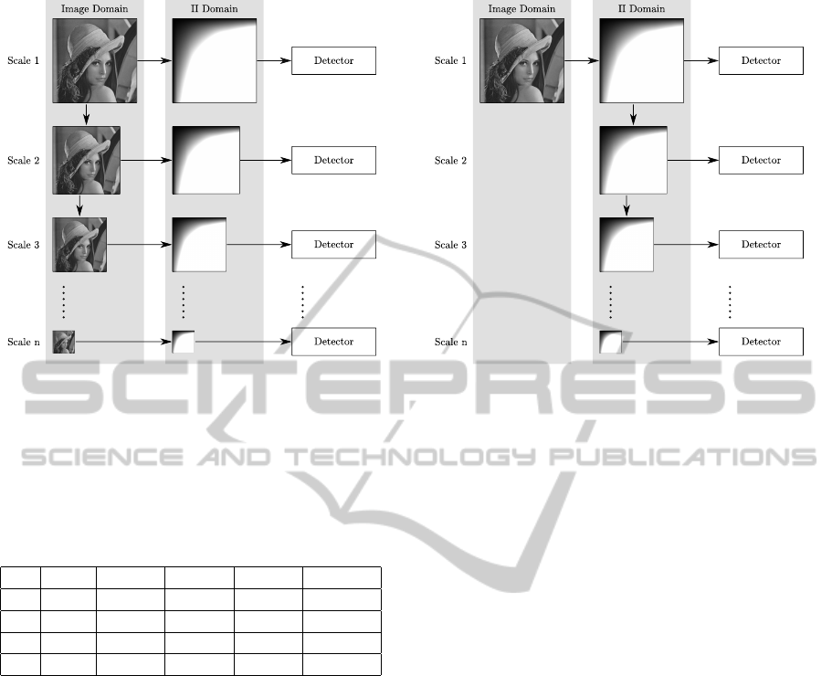
Figure 5: Illustration and comparison of OpenCV’s multi-scale LBP detector (left) and our modification of it (right). By using
the proposed integral image resizing approach, our modification does not require the recalculation of the integral images on
each scale.
Table 2: Dependency of integral image calculation time at
lower scales of the LBP detector on the number of available
CPU cores n. All values are relative to the detector’s to-
tal execution time for the respective hardware and software
configuration.
n SYS AVG SDEV MIN MAX
1 A
∗
2.9% 0.71% 1.57% 6.78%
2 A 4.66% 0.66% 2.92% 6.89%
4 B
∗∗
6.38% 0.78% 4.38% 9.87%
64 C 12.6% 4.86% 4.21% 37.25%
∗
TBB support disabled
∗∗
2 cores with hyper-threading
clearer when considering test system C with 64 total
CPU cores with an average and maximum speedup of
12.6% and 37.25%, respectively.
Note that our modification also allows speeding
up the overall detection process when TBB support in
OpenCV is disabled, i.e., when only one CPU core is
actually used. This can be seen in the corresponding
row in table 2 which reveals an average speedup of
2.9% in this case. However, it is not recommended
to only use one CPU core when more are available as
a higher number of CPU cores increases the speedup
significantly as shown above.
5 CONCLUSIONS
We proposed a new approach for image resizing
which works entirely in the integral image domain.
For the special case of power-of-two resizing, we pre-
sented a highly parallelizable version of our approach
which requires only a quarter of the operations com-
pared to regular bilinear interpolation in the image
domain, but provides the same exact results. Further-
more, we evaluated the practicality of our general ap-
proach by modifying one of multiple state-of-the-art
multi-scale integral-image-based object detection al-
gorithms in OpenCV without degrading its detection
performance. In total, a speed-up of an average of
6.38% and 12.6% could be achieved on a dual-core
mobile computer and a multi-processor server, re-
spectively. Moreover, we showed that similar results
can be achieved for all multi-scale integral-image-
based object detection algorithms.
ACKNOWLEDGEMENTS
This work is supported by FFG Bridge project
832082.
REFERENCES
Ahonen, T., Hadid, A., and Pietik
¨
ainen, M. (2004). Face
Recognition with Local Binary Patterns. In Pajdla, T.
and Matas, J., editors, Computer Vision – ECCV 2004,
volume 3021 of Lecture Notes in Computer Science,
pages 469–481. Springer Berlin Heidelberg.
Bay, H., Ess, A., Tuytelaars, T., and Van Gool, L. (2008).
Speeded-up robust features (surf). Comput. Vis. Image
Underst., 110:346–359.
SpeedingUpObjectDetection-FastResizingintheIntegralImageDomain
71

Bilgic, B., Horn, B. K., and Masaki, I. (2010). Efficient in-
tegral image computation on the GPU. In 2010 IEEE
Intelligent Vehicles Symposium (IV), pages 528–533,
San Diego, CA, USA. IEEE.
Crow, F. C. (1984). Summed-area tables for texture map-
ping. In Proceedings of the 11th annual conference on
Computer graphics and interactive techniques, SIG-
GRAPH ’84, pages 207–212, New York, NY, USA.
ACM.
Heckbert, P. S. (1986). Filtering by repeated integra-
tion. In Proceedings of the 13th annual conference on
Computer graphics and interactive techniques, SIG-
GRAPH ’86, pages 315–321, New York, NY, USA.
ACM.
Hensley, J., Scheuermann, T., Coombe, G., Singh, M., and
Lastra, A. (2005). Fast Summed-Area Table Genera-
tion and its Applications. Computer Graphics Forum,
24(3):547–555.
Hussein, M., Porikli, F., and Davis, L. (2008). Kernel in-
tegral images: A framework for fast non-uniform fil-
tering. In IEEE Conference on Computer Vision and
Pattern Recognition 2008 (CVPR 2008), pages 1–8,
Anchorage, AK, USA. IEEE.
Intel (2012). Intel 64 and IA-32 Architec-
tures Software Developer’s Manual, Vol-
ume 2B: Instruction Set Reference, N-Z.
http://www.intel.com/Assets/PDF/manual/253667.pdf.
Seshadrinathan, K., Soundararajan, R., Bovik, A., and Cor-
mack, L. (2010). Study of Subjective and Objective
Quality Assessment of Video. IEEE Transactions on
Image Processing, 19(6):1427–1441.
Viola, P. and Jones, M. (2001). Robust Real-time Object de-
tection. In International Journal of Computer Vision,
volume 57, pages 137–154.
Willow Garage (2012). OpenCV. http://opencv.
willowgarage.com/.
Yu, C., Dian-ren, C., Xu, Y., and Yang, L. (2010). Fast Two-
Dimensional Otsu’s Thresholding Method Based on
Integral Image. In 2010 International Conference on
Multimedia Technology (ICMT), pages 1–4, Ningbo,
China. IEEE.
VISAPP2014-InternationalConferenceonComputerVisionTheoryandApplications
72
