Eye-tracking Investigation During Visual Analysis of Projected

Multidimensional Data with 2D Scatterplots

Ronak Etemadpour, Bettina Olk and Lars Linsen

Jacobs University Bremen, Bremen, Germany

Keywords:

Projections, Dimensionality Reduction, Multidimensional Data, Perception-based Evaluation, Eye Tracking.

Abstract:

A common strategy for visual encoding of multidimensional data for visual analyses is to use dimensionality

reduction. Each multidimensional data point is projected to a 2D point using a certain strategy for the 2D

layout. Many layout strategies have been proposed addressing different objectives and targeted at distinct

domains and applications. The resulting projected information is typically displayed in form of 2D scatterplots.

The user’s perspective such as the role of visual attention and guidance of attention for a respective layout and

task has not been addressed much. It is the goal of this work to investigate, how characteristics in the layout

affect the cognitive process during task completion. Eye trackers are an effective means to capture visual

attention over time. We use eye tracking in a user study, where we ask users to perform typical analysis tasks

for projected multidimensional data such as relation seeking, behavior comparison, and pattern identiﬁcation.

Those tasks often involve detecting and correlating clusters. To understand the role of point density within

clusters, cluster sizes, and cluster shapes, we ﬁrst conducted a study with synthetic 2D scatterplots, where

we can set the respective properties manually. We evaluate how changing various parameters affect the visual

attention pattern and correlate it to the correctness of the answer. In a second step, we conducted a study where

the users were asked to complete tasks on real-world data with different characteristics (image collection and

document collection) that are visualized using a selection of different dimensionality reduction algorithms.

We transfer the insight obtained from synthetic data to investigate the decision making with real-world data.

Gestalt laws can be applied to the layout structure. We examine how certain layout techniques produce certain

characteristics that change the visual attention pattern. We draw some conclusions on how different projection

methods support or hinder decision making leading to respective guidelines.

1 INTRODUCTION

The goal when analyzing multidimensional data is to

identify structures in the data distribution. By multi-

dimensional data we refer to sets of points in a mul-

tidimensional space. Typical analysis tasks for gain-

ing insight into the properties of data distribution in-

clude pattern identiﬁcation such as detecting clusters,

behavior comparison such as comparing characteris-

tics of subsets, and relation seeking such as corre-

lating subsets to each other, see Section 3. For a

visual analysis of multidimensional data, it is com-

mon to use dimensionality reduction techniques that

project the multidimensional points to points in a

lower-dimensional visual space and typically, the pro-

jected points are displayed in form of 2D scatterplots.

Since one is interested into gaining insight in data

distributions in the multidimensional space, the pro-

jection method shall preserve those distributions as

much as possible. In general, it cannot be avoided

that some information is lost when reducing dimen-

sionality. Therefore, different projection techniques

have been established that focus on preserving cer-

tain properties of the data distribution. Consequently,

they aim at supporting certain analysis tasks where

those properties are crucial. To evaluate the effec-

tiveness of preserving certain properties, various nu-

merical and visual methods have been introduced to

quantify the quality of projections with respect to pre-

serving certain properties, thus, guiding a user to se-

lect the most appropriate projection method for their

task (Sips et al., 2009). Commonly, one consid-

ers cluster preservation or separation, neighborhood

preservation, or distance preservation properties. Per-

ceptional aspects have not been in the focus of at-

tention very much. Although projection techniques

are commonly embedded into user-centric systems

for interactive visual analysis, little is known about

how users perceive the layouts they produce. Typi-

cal perceptional questions would be how point den-

sity within a cluster, cluster size, and cluster shapes

affect the visual attention of an observer during the

233

Etemadpour R., Olk B. and Linsen L..

Eye-tracking Investigation During Visual Analysis of Projected Multidimensional Data with 2D Scatterplots.

DOI: 10.5220/0004675802330246

In Proceedings of the 5th International Conference on Information Visualization Theory and Applications (IVAPP-2014), pages 233-246

ISBN: 978-989-758-005-5

 2014 SCITEPRESS (Science and Technology Publications, Lda.)

analysis process and how this guidance of attention

relates to the provided answer. Automatic clustering

algorithms that compute partitions of points into sub-

sets or classes in order to maximize both the similarity

among members of the same subset, and dissimilar-

ity across classes are commonly embedded in a visual

analytics setting. On the other hand, Gestalt psychol-

ogists have studied grouping as part of the general

process of perception (KotBca, 1935) and formulated

a set of laws to explain the perceptual processes of

grouping done by humans. Our goal is to investigate

how perceptual aspects inﬂuence visual analyses.

In this paper, we present a study that investigates

visual attention during the analysis of multidimen-

sional data when projected to a two-dimensional vi-

sual space and visually encoded as 2D scatterplots.

Four types of seeing with different levels of attention

have been introduced by Wolfe (Wolfe, 2000). Previ-

ous research has demonstrated a strong link between

attention and eye movements based on the “eye-mind

hypothesis” (Rayner, 1998). Thereby, to assess the

allocation of visual attention, eye movement patterns

were recorded. Visual attention can be inﬂuenced by

many factors. Creating multidimensional data pro-

jection outputs where exactly one of these factors

varies is impossible. Thus, in a ﬁrst step we ana-

lyze eye movements when given typical analysis tasks

for 2D scatterplots that have been generated manually.

Eye movement patterns are analyzed in order to infer

where visual attention was allocated. For such syn-

thetic examples, we can tune respective parameters

such as point density, cluster size, or cluster shapes.

We analyze the impact of such parameters on relation-

seeking tasks, see Section 4.

In a second step, we use actual multidimensional data

sets from two different applications (image collec-

tions and documents collections) and project the data

to two-dimensional visual spaces using different point

placement techniques. Users are asked to perform

typical analysis tasks on the resulting 2D scatterplots

including the relation-ﬁnding tasks used for synthetic

data. We investigate the users’ eye movement patterns

recorded with the eye-tracking system, relate those

patterns to the ﬁndings with synthetic data, and cor-

relate the patterns to the correctness of the given an-

swers for the questions asked. We draw conclusions

on how the different projection methods inﬂuence vi-

sual attention and how this supports or hinders cor-

rect task completion, see Section 5. Our two-step ap-

proach follows the reasoning of Ware (Ware, 2000)

who discusses that the results of low-level processing

and discovering patterns can provide design guide-

lines for display layouts. The results of our ﬁrst step

can be applied to understand how existing layouts are

processed in our second step.

2 RELATED WORK

Many techniques exist to generate 2D similarity-

based layouts from high-dimensional data (projec-

tions). The design goals include maintaining pairwise

distances between points as implemented in multidi-

mensional scaling (MDS) (Borg and Groenen, 2010),

maintaining distances within a cluster, or maintain-

ing distances between clusters (Tenembaum et al.,

2000). Isometric feature mapping (Isomap) (Tenem-

baum et al., 2000) is an MDS approach that has been

introduced as an alternative to classical scaling ca-

pable of handling non-linear data sets. It obtains

a globally optimal solution to the distance preser-

vation problem. Classical dimensionality reduction

algorithms, such as principal component analysis

(PCA) (Jolliffe, 1986), are often employed to gen-

erate similarity layouts by reducing data to lower-

dimensional visual spaces. Least Square Projection

(LSP) (Paulovich et al., 2008) ﬁrst samples a reduced

sub-set of points representative of the data distribu-

tion in the input space and projects them to the target

space with a precise MDS force placement technique.

It then builds a linear system from information given

by the projected points and their neighborhoods. A

Laplacian operator ensures that data points in a par-

ticular neighborhood remain proximate in the target

space. They are based on ﬁrst generating a tree that

encodes similarity and then laying out the tree in a

two-dimensional space. The algorithms to generate

similarity layouts (Cuadros et al., 2007) are often

inspired by the neighbor-joining (NJ) heuristic orig-

inally proposed to reconstruct phylogenetic trees.

Several approaches for selecting good layouts have

been proposed. The approaches can be categorized

into numerical approaches that compute quality mea-

sures in form of numbers or visual approaches that

plot quality measures in graphical form. The silhou-

ette coefﬁcient (Tan et al., 2005) and the neighbor-

hood hit (Paulovich et al., 2008) evaluate clustering

capability, while the correlation coefﬁcients (Geng

et al., 2005) evaluate distances. These mathematical

measures do not consider how humans perceive the

layout.

User perception by conducting user studies on scat-

terplots is investigated in (Tatu et al., 2010). Users

were asked to sort useful scatterplots among 18 in-

stances. However, they did not look into multi-

dimensional data projection as the ones mentioned

above. A research by (Albuquerque et al., 2011),

is attempted to ﬁnd a perception-based quality mea-

IVAPP2014-InternationalConferenceonInformationVisualizationTheoryandApplications

234

sure for scatterplots. A ranking function was used

to estimate the value of the projections for a spe-

ciﬁc user task in a perceptual sense, based on the

data from a psychophysical study. Recently in (Sedl-

mair et al., 2012), the accuracy of class consistency

measure (CCM) and class density measure (CDM)

are discussed in scatterplots depicting multidimen-

sional projection layouts. Their major contribution

is a detailed taxonomy of factors that affect the hu-

man perception of cluster separation. In their quali-

tative data study, two investigators visually inspected

over 800 plots to determine whether or not the mea-

sures created plausible results. In a study by (Rensink

and Baldridge, 2010), the perception of correlation in

scatterplots has been investigated purely from a psy-

chological perspective developed for simple proper-

ties such as brightness. They generated a set of scat-

terplots with points distributed within a certain range

from the diagonal and tested whether observers could

discriminate pairs and concluded that perception of

correlation in a scatter plot is rapid. None of these ap-

proaches used eye trackers to measure visual attention

and draw conclusion on users’ decisions.

Eye tracking has been a helpful tool to understand the

cognitive processes of users involved in a visual anal-

ysis process. Eye tracking is used in (Burch et al.,

2011), to investigate the visual behavior of partici-

pants of a user study when operating with different

tree visualizations. They examined hierarchical struc-

tures represented by various tree layouts such as tradi-

tional, orthogonal, and radial node-link layouts. They

examined ﬁxation points, ﬁxation duration, and sac-

cades of participants’ gaze trajectories. They also an-

alyzed correctness of answers as well as completion

times in addition to the eye movement data. A similar

eye tracking study in (Goldberg and Helfman, 2011)

is conducted to compare radial and linear graphs to

support lookup tasks for one and two data dimen-

sions. The tasks of both studies, however, are more

concerned with topological distances of nodes (with

respect to the tree topology) than with Euclidean dis-

tances of nodes in the layout. Hence, tasks, data, and

visual encoding are different from our study.

There has also been some fundamental work on the

Gestalt principles within the cognitive psychology

community that relate to our work. The Gestalt prin-

ciples describe psychological phenomena underlying

human perception of given tasks by viewing them as

organized and structured wholes. For the detection

of non-spherical clusters, various researchers sought

more robust ways to identify arbitrarily shaped clus-

ters rather than the sum of their constituent parts

computationally. Ahuja and Tuceryan (Ahuja and

Tuceryan, 1998) studied a computational approach

presented to extracting basic perceptual structures or

the lowest level grouping in dot patterns with the

goal to extract the perceptual segments of dots due

to their relative locations. Dots were assigned percep-

tual roles of interior dots, border dots, curve dots, and

isolated dots. Other studies investigated detection of

dotted lines in a noisy background consisting of dy-

namic patterns of identical dots (Uttal et al., 1970).

We considered in the ﬁrst part of our study the work

on perceptual organization.

3 MULTIDIMENSIONAL DATA

ANALYSIS TASKS

We ﬁrst identify multidimensional data analysis

tasks for scatterplot visualizations in a projected

2D space. In a framework proposed by Andrienko

and Andrienko (Andrienko and Andrienko, 2005)

synoptic visual analysis tasks have been grouped

into pattern identiﬁcation, behavior comparison, and

relation seeking. Within this framework, we identify

typical analysis tasks for multidimensional data. A

relation-seeking task is to investigate the similarities

between subgroups (clusters or individual objects).

We hence asked participants to:

Q1 Identify the closest cluster to a given object.

Q2 Identify the closest cluster to a given cluster.

In both tasks we try to determine whether the

green or the blue cluster is closer to the red object(s).

The colors blue and green are assigned randomly to

the clusters to avoid any bias towards a speciﬁc color.

In order to assess pattern identiﬁcation, partici-

pants were asked to:

Q3 Estimate the number of clusters.

Here, all points are colored in the same color

(blue) as shown in the example in Figure 7.

A behavior comparison task is to compare char-

acteristics of subsets (or clusters). In other words, we

try to examine whether the objects within one cluster

are more similar to each other than the objects within

another cluster. Thus, we ask the subjects to compare

the point densities within clusters, where density is

deﬁned as the number of points per area. The task is

deﬁned as:

Q4 Rank clusters by density.

Eye-trackingInvestigationDuringVisualAnalysisofProjectedMultidimensionalDatawith2DScatterplots

235

Here, we identify three clusters in the multidimen-

sional data set and color-code the respective projected

points in the 2D scatterplot using red, green, and blue

color, correspondingly. Again, the colors are assigned

randomly.

4 SYNTHETIC DATA STUDY

In the ﬁrst part of our study, we want to investigate the

role of certain cluster properties on visual attention

and task completion success. One of the modern psy-

chological rules that was applied to visual and pattern

perception is called Gestalt approaches (Wertheimer,

1923). Our goal is to examine whether it is just (Eu-

clidean) distances that matter when visually analyzing

the scatterplots or whether there are other character-

istics of the clusters that inﬂuence the visual analy-

sis from a perceptional view. The characteristics we

investigated were cluster density (i.e., point density

within a cluster as deﬁned above), cluster size (i.e.,

the number of objects or points that belong to a clus-

ter), and cluster shape (e.g., whether a cluster appears

to be round or elongated). The synthetic scatterplots

have been inspired by observations from real scatter-

plots.

4.1 Gestalt Laws

We formulate hypotheses based on Gestalt

laws (Wertheimer, 1923) and test the hypothe-

ses within a user study. We want to provide a short

description of the four Gestalt laws that we used.

Gestalt theory is based on the concept that the whole

is greater than the sum of its parts. Broad observation

initially identiﬁed about human perception led to a

number of laws about how humans perceive groups

of related information visually: (1) Law of Similarity:

Objects that have similar appearance are perceived

as a group. (2) Law of Proximity: Objects that share

spatial proximity are perceived as a group. (3) Law

of Continuity: Objects that are aligned are perceived

as a group. (4) Law of Closure: Objects that are

perceived to form a closed contour are treated as a

group.

4.2 Hypotheses

Considering Task Q1 that compares distances be-

tween a point and a cluster (set of points), the Law

of Proximity would postulate that the point is percep-

tually grouped with the closer cluster. Here, the clus-

ters have equal size to the point and we consider the

case that one of the cluster is denser than the other.

The Law of Similarity leads to the assumption that the

point would be grouped to the less dense (or sparser)

cluster, as the distance of the point to the clusters is

closer to the distances within the sparser cluster than

those within the denser cluster. We expect that visual

attention is drawn towards the sparse cluster. Hence,

we formulate the hypothesis:

H1. Sparser clusters are looked at for a longer overall

time and are considered closer to the given reference

object.

Similar results we expect for Task Q2. However, here,

the single reference object is replaced by a third ref-

erence cluster, which itself has a certain point density.

Thus, we may assume from the Law of Similarity that

the cluster whose density is more similar to the den-

sity of the reference cluster is more likely to be chosen

as being closer. We phrase the hypothesis:

H2. Visual attention and decision is affected by the

density of the reference cluster.

The inﬂuence of cluster shape on the given tasks can

be described with respect to the Law of Continuity. It

can be assumed that a reference point (or cluster) ap-

pears closer to a cluster, if it is located in the contin-

uation of that cluster’s principal direction, i.e., being

aligned with it. On the other hand, if the reference

point (or cluster) is located in a direction orthogonal

to the principal direction, it is expected to appear far-

ther. Consequently, we formulate the hypothesis:

H3. Reference points (or clusters) appear closer to

clusters they are aligned with.

To test for the inﬂuence on cluster size, we use two

clusters of same shape and density and varied size

(i.e., the number of points). Based on the Law of Con-

tinuity, we assume that the reference point (in Task

Q1) or cluster (in Task Q2) is more likely to be per-

ceptually merged with the larger cluster. Hence, we

formulate the hypothesis:

H4. Reference points (or clusters) appear closer to

larger clusters.

4.3 Design of User Study

In a study on perception of random dot interference

patterns (Glass et al., 1973) is shown that varying

both the local and global parameters describing the in-

terference patterns, the functional organisation of the

visual system can be probed and new perceptual af-

fects discovered. In a study by (Healey et al., 1996),

is stated that if a visualization tool was being used

to display multiple independent data values, interfer-

ence among features should ideally be eliminated. If

a visualization tool was being used to investigate a

speciﬁc relationship, like ﬁnding similarity here, the

“strongest” feature should be used to encode that re-

IVAPP2014-InternationalConferenceonInformationVisualizationTheoryandApplications

236

lationship. Secondary features used to encode addi-

tional data values must not interfere with the task-

relevant feature. Thus, we needed examples where

only one of the parameters varies while the others re-

main constant. As it is impossible to obtain projec-

tions of multidimensional data into a 2D visual space,

where exactly one of the parameters cluster density,

cluster size, and cluster shape varies, we manually

generated 2D scatterplots.

We created 20 synthetic images that show scatterplots

with manually deﬁned properties. The images are tar-

geted at the evaluation with respect to Tasks Q1 and

Q2. We deﬁne two clusters that are equally far (with

respect to the 2D Euclidean distance) from a reference

point (Q1) or a third reference cluster (Q2). Hence, if

only distances matter, we expect that subjects in about

50% of the cases choose the ﬁrst cluster and in about

50% of the cases choose the second cluster as being

closer to the reference point (or cluster). However,

we modify the characteristics of the two clusters, i.e.,

they differ in density, in size, or in shape. We also

added a control scatterplot image, where all param-

eters (density, size, and shape) are identical for both

clusters. The scatterplots are generated by deﬁning

shape and number of points per clusters and, then,

randomly placing the points inside the shape.

We conducted a controlled user study involving 20

subjects (12 female and 8 male) with different edu-

cational background and normal vision. We did not

provide any statistical analysis across the gender. The

subjects were not familiar with visual multidimen-

sional data analysis, but received a short introduction.

Based on their assigned study ID, each subject was

presented ten (Task Q1) or twelve (Task Q2) images

with 2D scatterplots. Each task was presented in writ-

ten form on a slide and subjects had the chance to

ask in case of any necessary clariﬁcation. The ex-

perimenter was present and manually recorded the

answers, which were given verbally by the subjects.

There was no time limit to fulﬁll the tasks.

During the experiment, a Tobii T60 eye tracking sys-

tem was used to record eye movements and sequences

of gaze ﬁxations of the subjects on the visuals. The

system consists of a 17-inch computer monitor with

a video camera built in which tracks the user’s eye

movements at 60 Hz. It did not constrain users’ mo-

tion allowing subjects to move freely and naturally

while they looked at the screen and answered ques-

tions. Each subject received a brief description of the

eye-tracking system. The data recording session be-

gan with an eye-tracking calibration, which consisted

of the user looking at the screen and following a mov-

ing dot with their eyes. Questions and scatterplot im-

ages were embedded in a slide show on the Tobii sys-

tem monitor.

4.4 Analysis Methods

To test for statistical signiﬁcance of deviations from

a theoretically expected distribution of observations

into two categories, two-tailed binomial tests have

been used. ANOVA test was used for computing sta-

tistical signiﬁcance when comparing more than two

groups.

To analyze the visual attention patterns we used

the EyeC software system (Ristovski et al., 2013). It

computes heat maps from ﬁxation durations, which

maps to each pixel a color ranging from blue (no ﬁx-

ation) to red (highest ﬁxation duration), see Figure 1

(mid). Moreover, the user can select AOIs and re-

trieve statistical information about them, see Figure 1

(right). It shows the difference between the accumu-

lated ﬁxation times for the selected areas of interest

(AOIs) and selected participants. The AOI labels in

the heat maps are inserted manually for the images

shown. The shapes are shown by their contours. Fi-

nally, one can also analyze visual attention sequence

encoded over deﬁned AOIs (not shown in the ﬁgure).

4.5 Results

Inﬂuence of Cluster Density. In our experiments for

Task Q1, we created six different scatterplots. Two

images show scatterplots where both clusters had the

same roundish shape and the same size, while the den-

sity varied, see Figure 1 (left). Since density is related

to size, we also looked into varying size in addition

to density and created two further images where the

denser cluster had more points and another two im-

ages where the denser cluster had less points. To an-

alyze the ﬁxation patterns, we deﬁned ﬁve AOIs: The

area around the reference object (AOI 1), the space

between the reference object and the sparser cluster

(AOI 2), the sparser cluster (AOI 3), the denser cluster

(AOI 4), and the space between the reference object

and the denser cluster (AOI 5), cf. Figure 1 (mid). We

selected those ﬁve AOIs, as we assumed that the cog-

nitive process includes examining the clusters to ﬁnd

the point closest to the reference point and examining

the respective distances to the reference point.

The ﬁndings showed that in all six scatterplots the

sparse cluster (AOI 3) were signiﬁcantly looked at

more than all the other AOIs, cf. Figure 1 (right). In

accordance with this ﬁnding, in 75.83% the sparser

cluster has been reported as the closer one by the 20

subjects, which is signiﬁcantly more than the to be

expected 50%. Hence, Hypothesis H1 is conﬁrmed.

At this point, we want to mention that for the control

Eye-trackingInvestigationDuringVisualAnalysisofProjectedMultidimensionalDatawith2DScatterplots

237

scatter plot, where both clusters have the same den-

sity, size, and shape, there was no signiﬁcant differ-

ence in the visual attention and the answers from the

expected 50%.

We can also conclude that density seems to be per-

ceptually more relevant than cluster size, as changing

the cluster size did not change the fact that the sparser

cluster got more attention. Another observation is that

the single point (AOI 1) did not need much attention,

where the ﬁxation durations sometimes were negligi-

ble. Also, AOI 5 was looked at more than AOI 2,

which means that the space between the dense clus-

ter and the single object was more recognizable. The

sequence analysis shows that eyes frequently moved

from AOI 3 to AOI 5, before proceeding to AOI 4.

Figure 1: Task Q1: Finding closest cluster to reference point

for synthetic data with varying cluster density.

The ﬁndings for Task Q2 revealed that in ﬁve

out of the six scatterplots subjects still looked at the

sparser cluster most, cf. Figure 2(a). Also, in 86.4%

of all cases subjects started their analysis by look-

ing at the sparser cluster, which is statistically sig-

niﬁcant. In some cases the reference cluster was ac-

tually looked at most. A general observation was

that the reference cluster got substantially more atten-

tion when moved to the center between the two other

clusters. Despite these ﬁndings, the answers that the

sparser cluster is closer dropped to 56,6%, which is

actually not statistically signiﬁcant anymore. While

for the example shown in Figures 2(a) the sparser

cluster was generally reported as closer, all subjects

reported the denser cluster to be closer in the exam-

ple shown in Figure 2(b). When looking at the vi-

sual attention, the sparser cluster has still the high-

est mean ﬁxation duration in example (b). However,

as opposed to example (a), in example (b) the space

between the reference cluster and the sparser clus-

ter (AOI 6) is actually looked at more than the space

between the reference cluster and the denser cluster

(AOI 5). (c) AOI 1 got substantially more attention

than AOI 2, i.e., the part closer to the reference cluster

is investigated more. Hence, the subjects recognized

AOI 6 more, which let them decide for the denser

cluster to be closer. Now, when investigating the ref-

erence cluster’s density in the examples, it can be

seen that in example (a) it seems closer to that of the

sparser cluster, while in example (b) it seems closer to

the denser cluster. Investigating all six different scat-

(a)

(b)

Figure 2: Task Q2: Examples of ﬁnding closest cluster to

reference cluster for synthetic data with varying cluster den-

sity.

terplots, Hypothesis H2 has been conﬁrmed.

Inﬂuence of Cluster Shape. We ﬁrst considered

Task Q1 and generated eight scatterplots that targeted

two investigations. First, we used two clusters, where

one was more roundish the other more longish, while

density and size were the same. With this set-up, we

placed the reference point in continuation of the more

longish cluster or orthogonal to that direction. Sec-

ond, we looked into two longish clusters, where one

was bent and the other straight. The bending may be

in the direction away or towards the reference point.

For the ﬁrst case, in 80.7% of the cases the sub-

jects chose the roundish cluster as the closer one,

which is what we expected. However, 75% of the sub-

jects looked at the longish cluster more. In the case

of a roundish and a longish cluster, where the refer-

ence point is in the continuation of the longish clus-

ters (is not shown here), in 100% of the cases the sub-

jects chose the longish cluster as the closer one, which

again is what we expected. Here, 50% of the total

subjects looked at the longish cluster most (among

all AOIs deﬁned as before). One may speculate that

the elongated structure requires more attention than

the more compact, roundish structure to comprehend

the shape. To follow up on this, we investigated two

longish structures with one being bent as shown in

Figure 3(a). Here, the more complicated structure,

i.e., the curved one, is again the one that is looked at

more. However, the straight cluster was the one that

was seen closer by all subjects. This may relate to the

Law of Closure, as the curved cluster seems to deﬁne

a closed area, to which the reference point does not

belong.

Finally, we investigate the role of orientation of

the bending. We have a similar set-up as in Fig-

ure 3(a), but now the bending is towards the reference

point, cf. Figure 3(b). In this case the reference point

would lie inside the closure of the curved cluster. On

IVAPP2014-InternationalConferenceonInformationVisualizationTheoryandApplications

238

the other hand, the reference point lies in the continu-

ation of the straight cluster. Hence, the Laws of Con-

tinuity and Closure are competing. The ﬁndings were

that the straight cluster (AOI2) has the highest ﬁxa-

tion time, but that in 71% of all cases the subjects

chose the curved cluster as the closer one.

Hence, we conclude that Hypothesis H3 was con-

ﬁrmed. When considering two longish clusters with

one of them being curved, the Law of Closure seems

to be dominant, i.e., the orientation of the bending is

most relevant for the decision. The visual attention

patterns do not deliver such a consistent view as for

the varying densities, but it seems that more compact

clusters need less attention.

(a)

(b)

Figure 3: Task Q1: Finding closest cluster to reference point

for synthetic data with varying cluster shape.

For Task Q2, we investigated four scatterplots

with the two set-ups from above. I.e., we consider one

more roundish and one more longish cluster, where

the reference cluster is either located in continuation

of the longish cluster or in an orthogonal direction.

For the case, where the reference cluster is in contin-

uation of the longish cluster, the longish cluster was

chosen as the closer one in 82.35% of all cases (which

is statistically signiﬁcant). Consistently, the space be-

tween reference cluster and longish cluster had less

attention than the space between reference cluster and

roundish cluster. For the case, where the reference

cluster is in direction orthogonal to the longish cluster,

the roundish cluster was chosen as the closer one in

87.5% of the cases (which is statistically signiﬁcant).

Consistently, the space between reference cluster and

roundish cluster had less attention than the space be-

tween reference cluster and longish cluster. We can

conclude that these results also approve Hypothesis

H3.

Inﬂuence of Cluster Size. For Task Q1, in 75% of

the cases the larger cluster is indeed chosen as being

closer to the reference point and the respective AOI

has the highest mean ﬁxation duration (which is sta-

tistically signiﬁcant). The reference cluster in some

cases actually got most attention. For Task Q2, even in

89% of the cases the larger cluster is chosen as being

closer to the reference cluster (which is statistically

signiﬁcant). However, we can report that the space to

the smaller cluster is looked at more than the space to

the larger cluster, which is consistent with our earlier

ﬁndings. We can conclude that Hypothesis H4 was

conﬁrmed.

5 REAL DATA STUDY

In the second part of the study, we investigate ac-

tual multidimensional data. We identiﬁed two ap-

plication ﬁelds, where the multidimensional data sets

exhibit different characteristics. The ﬁrst application

is the visual analysis of document collections. Each

document represents an object. The corresponding

multidimensional point is a feature vector that rep-

resents the frequency of occurrences of certain key-

words in the document. The second application is the

visual analysis of image collections. Each image rep-

resents an object and the corresponding multidimen-

sional point is a vector of features that are derived

from the image using image processing steps. Doc-

ument data are typically of very high dimensional-

ity when compared to the number of objects, which

imposes a certain data sparseness. Image data are

typically of signiﬁcantly lower dimensionality, which

leads to a generally denser distribution.

5.1 Hypotheses

Considering distance-based tasks on real data, we can

formulate the following hypothesis based on the ﬁnd-

ings of the preceding section:

H5. Cluster density, shape, orientation, and size in-

ﬂuence distance estimation.

Next, we look into how visual attention matches the

analysis tasks. For cluster identiﬁcation, we formu-

late the hypothesis:

H6. There is a strong correlation between the visual

attention pattern (locations of AOIs) and the provided

answer when trying to identify clusters.

Concerning density-based tasks, we assume that

sparser clusters get more visual attention, based on

the ﬁndings of the preceding section. As the densities

of the clusters are examined in 2D scatterplots, the

densities in projected space are the ones that inﬂu-

ence the perception. How well the answers match the

cluster densities computed in high-dimensional space

also depends highly on how well the projection meth-

ods manage to maintain the cluster density properties

during projection. Our hypothesis is the following:

Eye-trackingInvestigationDuringVisualAnalysisofProjectedMultidimensionalDatawith2DScatterplots

239

H7. The sparser the clusters in the scatterplot, the

higher the visual attention.

5.2 Design of User Study

We picked four techniques as representatives of mod-

ern and classic strategies for embedding data in two

dimensions. Principal component analysis (PCA) has

been included in the study because it is a classical di-

mension reduction strategy often employed to gen-

erate visual embeddings of data. Isomap is effec-

tive on data that present non-linear relationships, that

both PCA and classical scaling typically fail to de-

tect. LSP is a modern dimension reduction technique

that presents precisely the results achieved with sam-

pling by clustering. Finally, we picked the neighbor-

joining (NJ) tree layout (Paiva et al., 2011) as a tree

layout for point placement to investigate whether their

good grouping and distance properties would be per-

ceived by users in the same way as the projections if

the edges are removed from the layouts (i.e., if visu-

ally encoded as a scatterplot).

We use two document and two image data sets.

The ﬁrst document data set - referred to as CBR - con-

tains 680 objects with 1,423 dimensions. The docu-

ment information includes title, authors, abstract, and

references from scientiﬁc papers in four different sub-

jects

. The second document data set - referred to as

KDViz - contains 1,624 objects with 520 dimensions

and four highly unbalanced labels generated from an

Internet repository

. The ﬁrst image data set - referred

to as Corel

- contains 1,000 objects with 150 dimen-

sions. The images are photographs on ten different

themes (Li and Wang, 2003). The second image data

set - referred to as Medical - contains 540 objects with

28 dimensions (features) including Fourier descrip-

tors and energies derived from histograms as well as

mean intensity and standard deviation computed from

the images themselves.

We conducted a controlled user study involving

the same subjects as above. Each subject was pre-

sented 56 images with 2D scatterplots of projected

multidimensional data using the four presented pro-

jection methods and asking one of the four identiﬁed

tasks. We had to exclude a few cases from our study

such as some tasks when PCA is applied to KDViz be-

cause of severe visual clutter that made it impossible

to identify clusters and AOIs. The set-up of the ex-

periments including eye tracking were as above. Ac-

tually, both parts (synthetic and real data) were exe-

cuted in one session. The entire experiment did not

http://vicg.icmc.usp.br/infovis2/DataSets

UCI KDD Archive, http://kdd.ics.uci.edu

take longer than 42 minutes for any of the subjects.

5.3 Analysis Methods

For the analysis of the correctness of the answers

using real data, we computed the ground truth (dis-

tances, densities, and clusters) in the multidimen-

sional space. Pairwise distances (Tasks Q1 and Q2)

are computed using cosine distances for document

data and Euclidean distances for image data to iden-

tify smallest distances. Clusters (Tasks Q1 and Q2)

were computed using an X-means approach (Pelleg

and Moore, 2000) and picking clusters with good

properties that adhere to the given labeling. Densi-

ties (Task Q4) are computed as the inverse of the av-

erage edge length in the minimum spanning tree of

each cluster, which is a simple distance-based mea-

sure that is sufﬁcient for comparative analysis. More-

over, it scales well to high dimensions, is not biased

towards any shape, and insensitive to density changes.

Statistical methods and eye tracking analysis methods

were the same as above.

5.4 Results

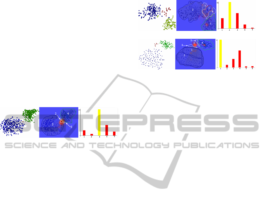
Closest Cluster to Reference Point. Task Q1 is

again concerned with the identiﬁcation of the closest

cluster to a reference point. However, now the refer-

ence point is not equally distant from the cluster. The

correct answer is computed in the high-dimensional

space before projection. Also, the clusters have been

computed before projecting. It is clearly visible from

the examples in Figure 4 that different projection

methods did differently well in preserving and sep-

arating the clusters. Also, there are severe difference

between the results of different data sets for the same

projection method. According to the mean correct-

ness of the given answers for Task Q1 considering

all dataset, LSP got the highest correctness (58.33%),

closely followed by Isomap (53.125%), while PCA

(19.79%) and Tree (9.375%) had lower correctness

and Anova test showed signiﬁcant difference among

them (P=0.034). We investigated visual attention and

cognitive processes for the individual examples. For

the scatterplots generated using Isomap we observed

a consistent visual attention pattern to our synthetic

data, as the sparser cluster was the most looked at

AOI, while the reference point got almost no atten-

tion. Figure 4(a) shows the example of Isomap ap-

plied to CBR, where we have two conﬂicting proper-

ties. The green cluster is sparser, but the blue cluster

is larger. According to our ﬁndings from synthetic ex-

amples, density was dominant over size. Here, how-

ever, the clusters are not completely separated and

IVAPP2014-InternationalConferenceonInformationVisualizationTheoryandApplications

240

only 37.5% of the subjects reported the green cluster

as closer, although this would have been the correct

answer.

For LSP the visual attention patterns when consid-

ering document data are similar to Isomap. However,

we observed interesting cases for the image data sets.

When LSP is applied to Corel, the reference point lies

in the continuation of the blue cluster and subjects fol-

lowed the Law of Continuity and incorrectly chose the

wrong cluster as the closer one. Correctness dropped

to 33.33%. In Figure 4(b), on the other hand, LSP is

applied to Medical, and the reference point is aligned

with the blue cluster. The Law of Continuity made

100% of the subjects choose correctly the blue cluster

as the closer one.

For PCA the clusters were generally not well pre-

served or separated, which led to lower correctness.

In Figure 4(c), for the Medical data set, 62.5% of

the subjects correctly reported the green cluster being

closer and it becomes evident that the green cluster is

the sparser one. Subjects followed our earlier identi-

ﬁed pattern, as the sparser cluster (AOI 2) is the AOI

with most visual attention. We want to note that for

some examples, we could only identify three mean-

ingful AOIs (reference point, cluster 1, cluster 2), as

it is not obvious what the space between the clusters

and the reference point would be.

The Tree layout created the least correct results for

Task Q1 on average. Figure 4(d) shows the worst case

when Tree is applied to Corel leading to 0% correct-

ness. The Tree layouts are, in general, most affected

by the Gestalt laws, as the generated branches - ac-

cording to the Law of Continuity - create the percep-

tion of a whole even when not drawing the edges of

the tree. In Figure 4(d), the reference point happens to

be included in a branch that otherwise contains only

points of the blue cluster. The reference point (AOI 3)

is not looked at explicitly, as it is perceived as being

part of the whole (the branch with the blue cluster).

Consequently, all subjects incorrectly answered that

the reference point is closer to the blue cluster. In

summary, we can conclude that also for real (i.e., pro-

jected multidimensional) data cluster properties inﬂu-

ence the answers of the subjects. Hence, Hypothesis

H5 is approved.

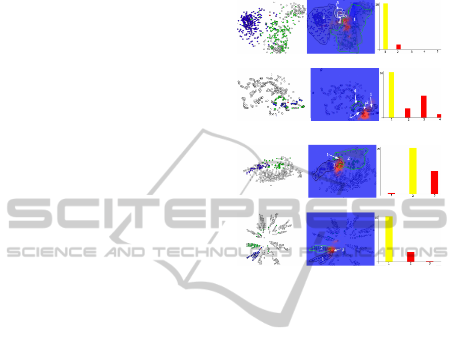
Closest Cluster to Reference Cluster. Task Q2 is

concerned with the identiﬁcation of the closest clus-

ter to a reference cluster. Again, ground truth is com-

puted in high-dimensional space. An additional as-

pect that comes in here is that the multi-dimensional

reference cluster itself may not be well preserved dur-

ing projection. For this task, we also want to test Hy-

pothesis H5.

(a) Isomap applied to CBR.

(b) LSP applied to Medical: Law of Continuity led to

correct answer.

(d) Tree applied to Corel.

Figure 4: Task Q1: Finding closest cluster to reference point

for real data.

Isomap was the projection method that created

best results in terms of correctness of the answers with

82.29% for the whole datasets. Again, the sparser

clusters are the AOIs that are observed most in al-

most all the cases. The only exception is shown in

Figure 5(a) when applied to Corel. Here the refer-

ence cluster is the one with higher mean ﬁxation dura-

tion. As it is shown, the red reference cluster actually

spreads over a large area of the scatterplot. It can fur-

ther be observed that the reference cluster mixes with

the green cluster. Based on the Proximity law, the

red and the green cluster are perceived as a whole and

accordingly 87.5% of the subjects selected the green

cluster as the closer one. Accumulated ﬁxation times

were higher for AOIs 3, 4, and 5 than for AOIs 1 and

LSP also produced good correctness values with

an average of 73.96%. The sparser clusters were

looked at most for all four data sets but the correctness

was lowest for the Medical data set. Investigating the

eye tracking data showed that the denser cluster also

got a large amount of attention for this example. The

reason why this example was often answered incor-

rectly is most likely the fact that the density of the

reference cluster matched the density of denser cluster

and based on the Law of Similarity, subjects reported

the denser cluster as the closer one incorrectly.

Eye-trackingInvestigationDuringVisualAnalysisofProjectedMultidimensionalDatawith2DScatterplots

241

PCA had the weakest performance on Task Q2

with a correctness of only 20.83%. Figure 5(b) gives

the example of PCA applied to Corel, which had a

correctness of 33.33%. The green cluster does not ex-

hibit a clear structure but is widely spread. AOI 3,

which represents the much more coherent and denser

blue cluster is examined longer. Although the refer-

ence cluster (AOI 2) is in proximity to both the green

and the blue cluster, its density is similar to the blue

cluster. According to the Law of Similarity this led

to the incorrect conclusion that the reference cluster

belongs to the blue cluster.

Tree layouts were correctly analyzed in 53.125%

of all cases. Least correct (0%) was the example when

Tree is applied to Corel, see Figure 5(d). Subjects

tend to investigate branches of the tree individually.

For example, AOIs 3 and 4 belong to the same cluster

but were not looked at sequentially. The same holds

true for AOIs 2 and 5. AOI 2 got the most visual at-

tention, which is based on the Law of Proximity, as it

is the one closest to the reference cluster. From the se-

quence of ﬁxations, one may even conclude that AOI1

and AOI2 were looked at together. Consequently, all

subjects answered incorrectly that the reference clus-

ter is closer to the blue cluster. In conclusion, Hy-

pothesis H5 was also conﬁrmed for Task Q2.

(a) Isomap applied to Corel.

(b) PCA applied to Corel.

Figure 5: Task Q2: Finding closest cluster to reference clus-

ter for real data.

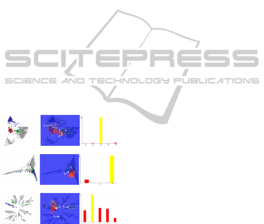
Cluster Identiﬁcation. Task Q3 is concerned

with identifying the clusters and reporting back the

number of identiﬁed clusters. According to the given

application, CBR had 4 labels (or classes), KDViz had

4 classes, Corel had 10 classes, and Medical had 12

classes, as indicated by the color coding in Figure 6.

However, when presenting the scatterplots to the sub-

jects, color coding of classes was removed. In the

following, we investigate how eye movement patterns

relate to the given answers. In particular, we look into

how many AOIs can be seen in the heat maps and

compare that to the answers given.

For Isomap we can state that the subjects’ answers

were close to their eye movement patterns. For CBR,

the subjects reported 3.5 clusters on average and we

could identify four hot spots (AOIs) in the heat map,

where the heat map result contains the eye movements

of all subjects. For KDViz, the heat map shows ﬁve

hot spots, while the average answer was four. We

further examine this case in Figure 6(a). In the se-

quence analysis, we observed a large amount of back-

and-forth movement between AOIs 1 and 2. Because

of the Laws of Proximity (AOIs 1 and 2 are close to

each other) and Similarity (AOIs 1 and 2 have sim-

ilar density), we can conclude that they have been

perceived as one cluster, which explains the answer

four instead of ﬁve. For Corel, seven hot spots can be

seen in the heat map and subjects reported 7.83 clus-

ters on average. For Medical, nine hot spots can be

seen in the heat map and subjects reported 9.89 clus-

ters on average. We can draw the conclusion that the

hot spots in the visual attention match very well the

answers that were given. However, the reported num-

bers are not necessarily the exact number of classes,

as the projection may fail to keep clusters sufﬁciently

separated. We observe that the reported numbers for

Isomap are lower or equal than the actual number of

classes. Moreover, the visual attention pattern reveals

that even when the correct answer is given, it may be

that the perceived clusters do not match the projected

classes. For example, in Figure 6(a), the blue and

red classes are highly overlapping and have been per-

ceived as one cluster, while the dark green class has

been split into two clusters. Consequently, the answer

is correct despite the two perceptual mismatches.

For LSP the answers also matched well the number

of hot spots. For CBR four hot spots were observed

and subjects reported 4.85 clusters on average, for

KDViz ﬁve hot spots were observed and subjects re-

ported 4.375 clusters on average, for Corel nine hot

spots were observed and subjects reported 11.14 clus-

ters on average, and for Medical eight hot spots were

observed and subjects reported 8.375 clusters on aver-

age. Obviously, for the examples with larger number

of clusters, it gets more difﬁcult to distinguish the hot

spots and identify AOIs. In Figure 6(b), we try to in-

vestigate some AOIs for the example of the Medical

data set. AOI 1 got most attention, as it is a sparser

structure that needs longer investigation to make a de-

cision. On the contrary, the dense cyan cluster in AOI

7 was obvious and did not need to be looked at in-

IVAPP2014-InternationalConferenceonInformationVisualizationTheoryandApplications

242

tensively. We also deduce that AOI 5 (despite being

quite dense) needs quite some attention because of its

complex, non-concave structure.

For PCA we obtained the following results: For

CBR three hot spots were observed and subjects re-

ported 2.67 clusters on average, for KDViz two hot

spots were observed and subjects reported 2.375 clus-

ters on average, for Corel three hot spots were ob-

served and subjects reported 3.0 clusters on average,

and for Medical six hot spots were observed and sub-

jects reported 4.12 clusters on average. Again, there is

a pretty good match between the visual attention pat-

tern and the number of reported clusters. However, it

becomes very obvious that the numbers are generally

lower for PCA. For example, looking at the ﬁxation

sequence when applying PCA to CBR, we can deduce

that overlapping areas were considered as one cluster,

which explains why we only had three hot spots and

on average 2.67 reported clusters. Perceptually merg-

ing these areas is reasonable, as they have similar den-

sity (Law of Similarity) and are well aligned (Law of

Continuity). The general problem of PCA is that it

does not manage very well to keep clusters separated.

The cluttered clusters are, then, perceived as a single

big cluster.

Finally, for Tree, subjects reported 11.64 clusters

for CBR, 13.875 clusters for KDViz, 10.875 clusters

for Corel, and 10.625 clusters for Medical. Obvi-

ously, numbers are generally higher for Tree. The

ﬁxation times reﬂect that the hot spots match the

branches of the tree layout. Figure 6(d) shows the ex-

ample of applying Tree to CBR. Groups that belong

to one class are perceptually separated when split to

two branches, e.g., AOIs 3 and 7. Hence, the general

problem of Tree is that it does not manage very well

to preserve clusters. Clusters are split over multiple

perceptionally separated groups.

We conclude that the visual attention pattern

matches well the given answers, which conﬁrms Hy-

pothesis H6. Moreover, we have seen that PCA and

Isomap produced better results in form of preserving

and segregating clusters during projection. PCA often

produces scatterplots, where clusters were not sep-

arated well, while Tree produces scatterplots, where

clusters were not well preserved, i.e., split over mul-

tiple clearly separated groups. Cluster separation and

segregation is a highly studied topic when using pro-

jections for multidimensional data visualization. A

commonly used quality measure which measures the

cohesion and separation between groups of objects

on the layout is the silhouette coefﬁcient (Tan et al.,

2005). Given an object p

, its cohesion a

is the av-

erage distance between p

and all other objects be-

longing to the same group as p

. Its separation b

(a) Isomap applied to KDViz.

(b) LSP applied to Medical.

(d) Tree applied to CBR.

Figure 6: Task Q3: Estimate number of clusters for real

data.

the minimum distance between p

and all the other in-

stances belonging to the other groups. The silhouette

coefﬁcient of a projection is obtained by averaging the

silhouette coefﬁcients of its n objects. Resulting val-

ues vary in the range -1 and 1, with 1 meaning that

groups are perfectly separated. When computing the

silhouette coefﬁcients for the four projection methods

when applied to the four data sets, Isomap and LSP in-

deed had on average the best values (0.215). PCA has

the worst average silhouette coefﬁcient (0.145) and

even a negative one for KDViz. Tree’s average sil-

houette coefﬁcient lies in between (0.19). Hence, the

silhouette coefﬁcient results conﬁrm our ﬁndings.

Cluster Ranking. For Task Q4, we asked the

subjects to compare the density of clusters in the

scatterplot. We picked three clusters in the multi-

dimensional space and encoded them visually using

red, green, and blue color. The subjects had to rank

them by density. We also assume that the visual at-

tention pattern matches the rankings reported by the

subjects. In general, we observe a visual attention

pattern where sparser clusters in the scatterplot get

looked at more. In 12 out of the 16 scatterplots that

were examined, the subjects started their investiga-

tion by looking at the sparsest cluster and, on average,

also had the longest ﬁxation duration for the spars-

est cluster. Also, the densest clusters were, on aver-

age, looked at least when comparing the ﬁxation dura-

tions of the three highlighted clusters. When trying to

match the answers to the visual attention pattern, we

can report that this worked best for Isomap, where in

33.33% of all cases the reported ranking matches pre-

cisely the ranking of average ﬁxation duration. For

the other methods the respective numbers are 29.16%

Eye-trackingInvestigationDuringVisualAnalysisofProjectedMultidimensionalDatawith2DScatterplots

243

for LSP, 24.10% for Tree, and 18.75% for PCA. When

only seeking the densest cluster, the match occurs in

41.67% for Isomap, 39.58% for both LSP and PCA,

and 37.05% for Tree. Considering the correctness of

the answers with respect to densities computed in the

multi-dimensional space, the results are as follows:

Isomap achieved highest correctness (65.62%), fol-

lowed by PCA (47.92%), LSP (46.88%), and ﬁnally

Tree (42.85%).

For the PCA projection, the sparser cluster in the

2D scatterplot is the one looked at most and is re-

ported by the subject as sparsest. However, in the

multidimensional space the sparsest cluster is actu-

ally the densest. The comparative density properties

among clusters are not preserved by PCA. For the

Tree layout, the cluster that spreads over the entire

scatterplot got the highest amount of visual attention.

However, since there are densely populated branches

the overall density of the cluster was rated as high.

Consequently, the majority of subjects answered it as

the densest. The outliers that are part of branches (e.g.

AOI 6 in Figure 6(c)) with dominantly yellow points

here are not perceived as outliers, as the respective

branches are seen as a whole.

In summary, we observed that the projection

method may change comparative density properties

of clusters. In the scatterplot, there was a tendency to

have more visual attention for sparser clusters, as it

was postulated in Hypothesis H7. However, this ten-

dency was not as strong as expected, as other factors

like cluster separation, size, and shape also inﬂuence

perception here.

6 CONCLUSIONS

We have presented a study on the role of visual atten-

tion when interpreting scatterplots that were obtained

by projecting multidimensional data into 2D visual

spaces. In a ﬁrst part of our study, we considered

synthetic scatterplots, which allowed us to vary only

one perceptual factor at a time. Our hypotheses made

use of the Gestalt Laws of Proximity, Similarity, Con-

tinuity, and Closure to postulate that cluster proper-

ties such as density, shape (and also orientation), and

size inﬂuence perception when interpreting distances

in scatterplot. Density turned out to be more inﬂu-

ential than size. For distance tasks, there was a clear

tendency that the space between the reference and the

perceptually farther cluster was looked at more than

the space between the reference and the perceptually

closer cluster. Our hypotheses were conﬁrmed. There

was a clear correlation between this visual attention

pattern and the given answer.

In a second part of our study, we formulated respec-

tive hypotheses for visual analyses of projected mul-

tidimensional data. Investigating the role of cluster

characteristics in real-world data, we were able to

also conﬁrm those hypotheses and we can conclude

that there are multiple factors that inﬂuence percep-

tion (or visual attention) and that perception plays an

important role in interpreting the scatterplots. We

also performed a comparative analysis of four pro-

jection methods on two types of data, which led to

some guidelines for their usage. In particular, conti-

nuity can inﬂuence the answers signiﬁcantly, where

the Tree layout was most affected by this due to the

branching structure. Isomap and LSP, on the other

hand, had a tendency to create more roundish clusters

(of course, with exceptions), which led to less mis-

interpretations. PCA had problems with cluster seg-

regation, while Tree had issues with cluster preserva-

tion. Hence, projection methods should also be inves-

tigated with respect to how well they maintain these

properties. For example, when two clusters are being

projected, where one is denser than the other, the pro-

jected denser cluster should also be denser than the

projected sparser cluster and not vice versa. We also

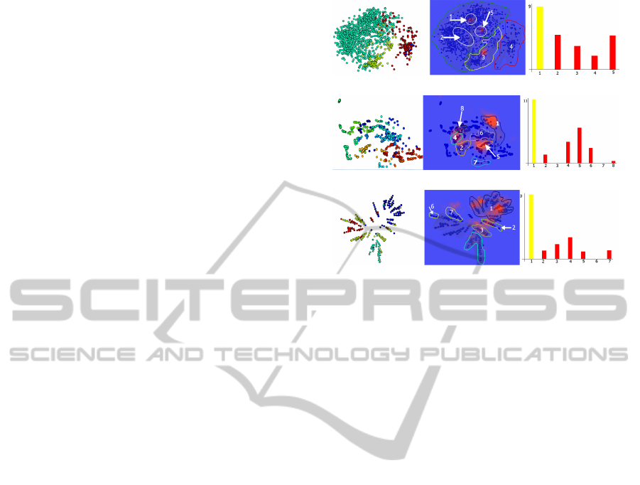
want to mention that we initially had included a ﬁfth

projection method in our study, namely Glimmer (In-

gram et al., 2009). In Glimmer iterative point place-

ment procedure is highly optimized by clever usage

of GPU hardware combined with a multilevel strat-

egy that operates on a hierarchical model of the un-

derlying particle-spring system. However, as shown

in the example in Figure 7, the projection and the vi-

sual attention pattern was scattered and we have not

been able to identify any meaningful AOIs for Glim-

mer and, therefore, excluded it from our study. The

silhouette coefﬁcients for Glimmer when applied to

our four data sets was negative.

Figure 7: Glimmer applied to CBR, overlaid with eye ﬁxa-

tion pattern for Task Q3 (using a green-to-red color map).

ACKNOWLEDGEMENTS

This work was supported by the research center on

Visual Communication and Expertise (VisComX) at

Jacobs University, Bremen, Germany as well as NSF

IVAPP2014-InternationalConferenceonInformationVisualizationTheoryandApplications

244

CCF-0808847. We would like to thank Eric Mon-

son, Rachael Brady, and Stephen Mitroff for their

kind help in conducting this study at Duke University,

Durham, USA.

REFERENCES

Ahuja, N. and Tuceryan, M. (1998). Extraction of early

perceptual structure in dot patterns: Integrating re-

gion, boundary, and component gestalt. Computer

Vision, Graphics, and Image Processing archive, 48

Issue:3:304–356.

Albuquerque, G., Eisemann, M., and Magnor, M. (2011).

Perception-based visual quality measures. In Proc.

IEEE Symposium on Visual Analytics Science and

Technology (VAST), pages 13–20.

Andrienko, N. and Andrienko, G. (2005). Exploratory

Analysis of Spatial and Temporal Data: A Systematic

Approach. Springer-Verlag New York, Inc., Secaucus,

NJ, USA.

Borg, I. and Groenen, P. J. F. (2010). Modern Multidimen-

sional Scaling Theory and Applications. Springer Se-

ries in Statistics. Springer, 2nd. edition edition.

Burch, M., Konevtsova, N., Heinrich, J., Hoeferlin, M., and

Weiskopf, D. (2011). Evaluation of traditional, or-

thogonal, and radial tree diagrams by an eye tracking

study. IEEE Transactions on Visualization and Com-

puter Graphics, 17(12):2440–2448.

Cuadros, A. M., Paulovich, F. V., Minghim, R., and Telles,

G. P. (2007). Point placement by phylogenetic trees

and its application to visual analysis of document col-

lections. In Proceedings of the 2007 IEEE Symposium

on Visual Analytics Science and Technology, pages

99–106. IEEE Computer Society.

Geng, X., Zhan, D. C., and Zhou, Z. H. (2005). Super-

vised nonlinear dimensionality reduction for visual-

ization and classiﬁcation. IEEE Transactions on Sys-

tems, Man, and Cybernetics, Part B: Cybernetics, 35

Issue:6:1098 – 1107.

Glass, L., Glass, L., and Perez, R. (1973). Perception of

random dot interference patterns. Nature 246, 1:360–

362.

Goldberg, J. H. and Helfman, J. (2011). Eye tracking

for visualization evaluation: Reading values on lin-

ear versus radial graphs. Information Visualization,

10(3):182–195.

Healey, B. G., Booth, K. S., and Enns, J. T. (1996). High-

speed visual estimation using preattentive processing.

ACM Transactions on Computer-Human Interaction,

3(2):107–135.

Ingram, S., Munzner, T., and Olano, M. (2009). Glimmer:

Multilevel mds on the gpu. IEEE Transactions on Vi-

sualization and Computer Graphics, 15(2):249–261.

Jolliffe, I. T. (1986). Pincipal Component Analysis.

Springer-Verlag.

KotBca, K. (1935). Principles of gestalt psychology, har-

court brace.

Li, J. and Wang, J. Z. (2003). Automatic linguistic indexing

of pictures by a statistical modeling approach. IEEE

Transactions on Pattern Analysis and Machine Intel-

ligence, 25(9):1075–1088.

Paiva, J. G. S., C., L. F., Pedrini, H., Telles, G. P., and

Minghim, R. (2011). Improved similarity trees and

their application to visual data classiﬁcation. IEEE

Transactions on Visualization and Computer Graph-

ics, 17(12):2459–2468.

Paulovich, F. V., Nonato, L. G., Minghim, R., and Lev-

kowitz, H. (2008). Least square projection: A fast

high-precision multidimensional projection technique

and its application to document mapping. IEEE

Transactions on Visualization and Computer Graph-

ics, 14(3):564–575.

Pelleg, D. and Moore, A. W. (2000). X-means: Extend-

ing k-means with efﬁcient estimation of the number

of clusters. In Proceedings of the 17th. International

Conference on Machine Learning, ICML ’00, pages

727–734, San Francisco, CA, USA. Morgan Kauf-

mann Publishers Inc.

Rayner, K. (1998). Eye movements in reading and informa-

tion processing: 20 years of research. Psychological

bulletin, 124(3).

Rensink, R. and Baldridge, G. (2010). The perception of

correlation in scatterplots. Computer Graphics Forum

(Proceedings of EuroVis 2010), 29:1203–1210.

Ristovski, G., Hunter, M., Olk, B., and Linsen, L. (2013).

Eyec: Coordinated views for interactive visual explo-

ration of eye-tracking data. In Proceedings of the

17th International Conference of Information Visual-

ization.

Sedlmair, M., Tatu, A., Munzner, T., and Tory, M. (2012).

A taxonomy of visual cluster separation factors. Com-

puter Graphics Forum (Proc. EuroVis), 31(3):1335–

1344.

Sips, M., Neubert, B., Lewis, J. P., and Hanrahan, P. (2009).

Selecting good views of high-dimensional data using

class consistency. In Hege, H.-C., Hotz, I., and Mun-

zner, T., editors, Eurographics/ IEEE-VGTC Sympo-

sium on Visualization 2009, volume 28 of Computer

Graphics Forum, pages 831–838, Berlin, Germany.

Blackwell.

Tan, P.-N., Steinbach, M., and Kumar, V. (2005). Intro-

duction to Data Mining. Addison-Wesley Longman,

Boston, MA, USA.

Tatu, A., Bak, P., Bertini, E., Keim, D. A., and Schnei-

dewind, J. (2010). Visual quality metrics and human

perception: an initial study on 2D projections of large

multidimensional data. In Proceedings of the Working

Conference on Advanced Visual Interfaces (AVI ’10),

pages 49–56.

Tenembaum, J. B., de Silva, V., and Langford, J. C. (2000).

A global geometric faramework for nonlinear dimen-

sionality reduction. Science, 290:2319–2323.

Uttal, W. R., Bunnell, L. M., and Corwin, S. (1970). On

the detectability of straight lines in visual noise: An

extension of French’s paradigm into the millisecond

domain. Perception & Psychophysics, 8:385–388.

Ware, C. (2000). Information visualization: perception for

design. Morgan Kaufmann Publishers Inc., San Fran-

cisco, CA, USA.

Eye-trackingInvestigationDuringVisualAnalysisofProjectedMultidimensionalDatawith2DScatterplots

245

Wertheimer, M. (1923). Untersuchungen zur Lehre von der

Gestalt. Psychological Research Psychological Re-

search, 4:301–350.

Wolfe, J. (2000). Visual attention. pages 335–386.

IVAPP2014-InternationalConferenceonInformationVisualizationTheoryandApplications

246