Calibrating Focal Length for Paracatadioptric Camera from One Circle
Image
Huixian Duan, Lin Mei, Yanfeng Shang and Chuanping Hu
R & D Center of Cyber-Physical Systems, The Third Research Institute of Ministry of Public Security,
Bisheng Road, Shanghai, China
Keywords:
Focal Length, Calibration, Paracatadioptric Camera, Circle Image.
Abstract:
Camera calibration from circles has great advantages, but for paracatadioptric camera, the estimation of in-
trinsic parameters using circle images is still an open and challenging problem. Previous work proved that
the paracatadioptric projection of a circle is a quartic curve. But due to the partial occlusion, only part of the
quartic curve is visible on the image plane. Consequently, circle image cannot be directly estimated using im-
age points extracted from the visible part and camera parameters cannot be calibrated. To solve this problem,
In this paper, we study the properties of paracatadioptric circle image and application in calibrating the focal
length for the case that aspect ratio is 1 and skew is 0. Firstly, we derive the necessary and sufficient conditions
that must be satisfied by paracatadioptric circle image. Next, based on these conditions, a new object function
is presented to correctly estimate the circle image. Then, we show that the focal length can be computed
from the estimated paracatadioptric circle image and the principal point that is estimated from the projected
contour of parabolic mirror. Experimental results on both simulated and real image data have demonstrated
the effectiveness of our method.
1 INTRODUCTION
Many applications in computer vision require that a
camera has a large field of view. Combining the
camera with mirrors, referred to as catadioptric im-
age formation, can increase the field of view of a
camera. According to the uniqueness of an effective
viewpoint, catadioptric systems can be classified into
two groups, central and noncentral (Baker and Nayer,
1999). Baker and Nayer (Baker and Nayer, 1999) in-
troduced that a central catadioptricsystem can be built
by combining an hyperbolic mirror with a perspective
camera, a parabolic mirror with an orthographic cam-
era, and planar mirror with a perspective camera. The
construction of the former requires a careful align-
ment between the mirror and the imaging device. But
the paracatadioptric camera is easier to construct be-
ing broadly used in vision applications.
Geyer and Daniilidis (Geyer and Daniilidis, 2001)
proposed a unifying model for general central cata-
dioptric image formation. It is shown that the imag-
ing process is equivalent to the two-step mapping by
a sphere. Under central catadioptric system, the cal-
ibration of camera is still a prerequisite for its ap-
plications. In the literature, the calibration methods
can be classified into the following four categories.
The first category (Aliaga, 2001; Wu and Hu, 2005;
Scaramuzza et al., 2006; Deng et al., 2007; Bastan-
lar et al., 2008) require a 3D/2D calibration pattern
with control points. The second category (Geyer and
Daniilidis, 1999; Geyer and Daniilidis, 2002; Barreto
and Araujo, 2002; Barreto and Araujo, 2003; Barreto
and Araujo, 2005; Barreto and Araujo, 2006; Geyer
and Daniilidis, 2002; Wu et al., 2006; Scaramuzza
et al., 2006; Wu et al., 2008; Duan et al., 2012) only
make use of the properties of line images. The third
category (Ying and Hu, 2004; Ying and Zha, 2008;
Duan and Wu, 2011a; Duan and Wu, 2012)is based
on the properties of sphere images. The fourth cate-
gory (Kang, 2000) only use point correspondence in
multiple views, without needing to know either the
3D location of space points or camera locations.
Camera calibration from circles has great advan-
tages. Especially, as a kind of central catadioptric
cameras, there have been many calibration methods
of the pinhole camera based on circle images in the
literature, and these methods can get high calibration
accuracy. However, due to large distortion, catadiop-
tric camera calibration from circle images has many
difficulties and lacks of studies. Based on the pro-
jection of a line complex, Sturm and Barreto(Sturm
and Barreto, 2008) proved that the central catadiop-
56
Duan H., Mei L., Shang Y. and Hu C..
Calibrating Focal Length for Paracatadioptric Camera from One Circle Image.
DOI: 10.5220/0004672800560063
In Proceedings of the 9th International Conference on Computer Vision Theory and Applications (VISAPP-2014), pages 56-63
ISBN: 978-989-758-003-1
Copyright
c
 2014 SCITEPRESS (Science and Technology Publications, Lda.)

tric projection of a quadric is a quartic curve. What’s
more, according to the imaging process under cen-
tral catadioptric model, Duan and Wu (Duan and Wu,
2011b) derived the algebraic expression of a circle
image and provided a unified imaging theory of dif-
ferent geometric elements, which established the the-
oretical foundation for calibration methods based on
circles. But due to the partial occlusion, only part of
the circle image is visible on the image plane. Conse-
quently, circle image cannot be directly estimated us-
ing image points extracting from the visible part and
camera parameters cannot be calibrated.
In this paper, for the case that aspect ratio is 1 and
skew is 0, we study the properties of paracatadiop-
tric circle image and application in calibrating the fo-
cal length. Firstly, the necessary and sufficient con-
ditions that must be satisfied by paracatadioptric cir-
cle image are derived. Secondly, these conditions are
used to correctly estimate the paracatadioptric circle
image. Finally, we show that the focal length can be
calibrated from the estimated paracatadioptric circle
image and the principal point that is estimated from
the projected contour of parabolic mirror. Experimen-
tal results on both simulated and real image data have
demonstrated the effectiveness of our method.
This paper is organized as follows: Section 2 re-
views the unified sphere model introduced by Geyer
and Daniilidis (Geyer and Daniilidis, 2001) and some
related works. Section 3 studies the properties of
paracatadioptric circle image. In section 4, the fo-
cal length is calibrated from one circle image and the
principal point. Experimental results are shown in
Section 5. Finally, Section 6 presents some conclud-
ing remarks.
2 PRELIMINARIES
A bold letter denotes a vector or a matrix. Without
special explanation, a vector is homogenous coordi-
nates. In the following, we briefly review the im-
age formation for paracatadioptric camera introduced
in (Geyer and Daniilidis, 2001), the antipodal image
points and their properties proposed in (Wu et al.,
2008) and the algebraic expression of paracatadiop-
tric circle image derived in (Duan and Wu, 2011b).
2.1 Paracatadioptric Projection Model
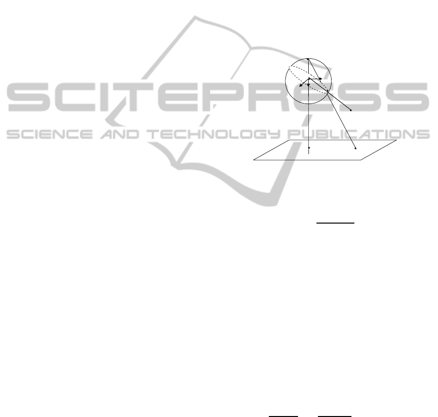
Geyer and Daniilidis (Geyer and Daniilidis, 2001)
showed that the paracatadioptric imaging process is
equivalent to the following two-step mapping by
a sphere (see Fig.1): Firstly, under the viewing
sphere coordinate system O− X
s
Y
s
Z
s
, a 3D point X =
(x, y, z)
T
is projected to a point X
s
= (x
s
, y
s
, z
s
)
T
on the
unit sphere centered at the viewpoint O; Secondly, the
point X
s
is projected to a point m on the image plane
Π by a pinhole camera through the perspective center
O
c
. The image plane is perpendicular to the line go-
ing through the viewpoints O and O
c
. Let the intrinsic
parameter matrix of the pinhole camera be
K
c
=


r
c
f
c
s u
0
0 f
c
v
0
0 0 1


where r
c
is the aspect ratio, f
c
is the effective focal
length, (u
0
, v
0
, 1)
T
denoted as p is the principal point,
and s is the skew factor.
m
p
c
O
O
X
s
X
s
X
s
Y
s
Z
Figure 1: The image formation of a point.
Then, the imaging process of a space point X to m
can be described as:
αm = K
c
(
RX+ t
kRX+ tk
+ e). (1)
where α is a scalar, R is a 3 × 3 rotation matrix, t
is a 3-vector of translation, k · k denotes the norm of
vector in it, e = (0, 0, 1)
T
.
2.2 The Antipodal Image Points
Under paracatadioptric camera, Wu et al. (Wu et al.,
2008) gave the definition of antipodal image points
and studied their properties as follows:
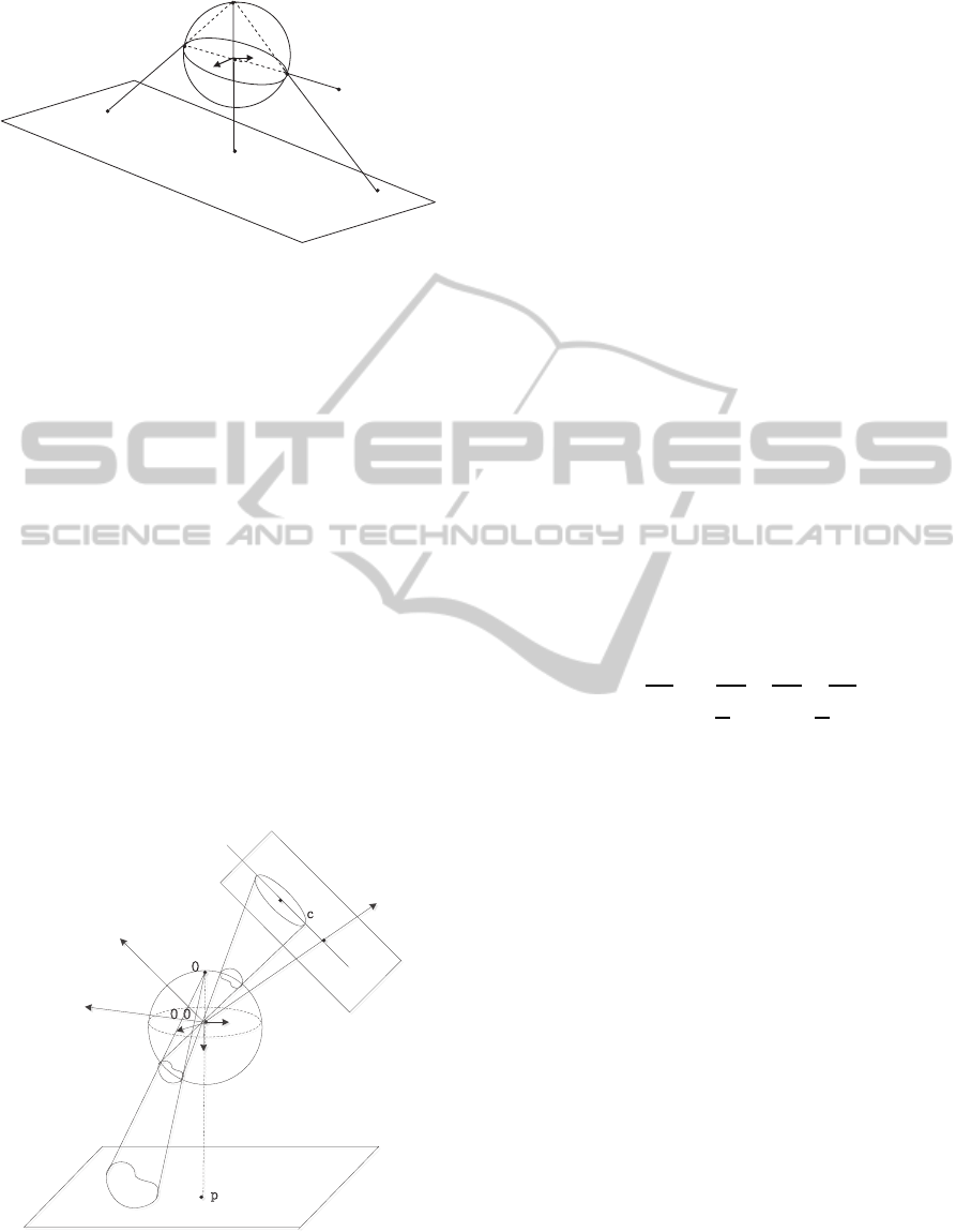
Definition 1. {m, m
′
} is called a pair of antipodal
image points if they could be images of two end points
of a diameter of the viewing sphere(See Fig.2).
Proposition 1. If {m, m
′
} is a pair of antipodal image
points under paracatadioptric camera, we have:
1
m
T
ϖm
m+
1
m
′
T
ϖm
′
m
′
= p. (2)
where ϖ= K
−T
c
K
−1
c
, and p is the principal point.
2.3 The Paracatadioptric Circle Image
Generally, the projection of a circle is a quartic curve
under paracatadioptric camera. Duan and Wu(Duan
CalibratingFocalLengthforParacatadioptricCamerafromOneCircleImage
57

s
Y
s
Z
O
m
'
m
p
s
X
c
O
X
Figure 2: {m, m
′
} is a pair of antipodal image points.
and Wu, 2011b) derived the algebraic expression of
circle image. In order to make this paper complete,
we show the detail as follows.
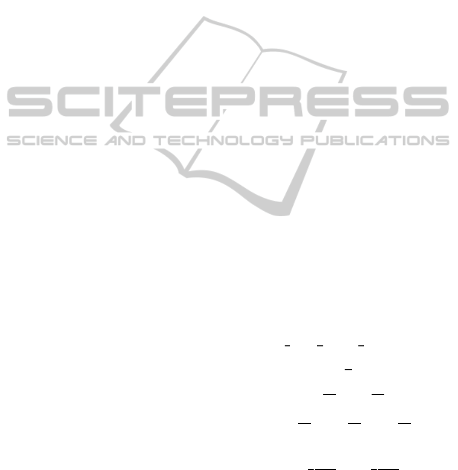
Firstly, set up the world coordinate system (see
Fig.3): O as the origin O
W
; the line through the ori-
gin O
W
and orthogonal to the plane containing c as
the Z−axis; the point where Z−axis and the plane
containing c intersect as the point o, the line through
the point o and center of c as the line l, then the line
through the origin O
W
and parallel to the line l as
X−axis; the line through the origin O
W
and orthog-
onal to the X−axis and Z−axis as Y−axis; denoted
as O
W
− X
W
,Y
W
, Z
W
. Then, under the world coordi-
nate system, the equation of the circle c is:

(x− x
0
)
2
+ y
2
= r
2
z = z
0
where z
0
is the distance from the origin O
W
to the
plane containing c, r is the radius of c, x
0
is the co-
ordinate of the center of c under the world coordinate
system.

:
22
F
2
S
F
o
W
Z
W
X
W
Y
s
Z
s
X
s
Y
l

x
Figure 3: The image formation of a circle.
Proposition 2. Let m be one image point on paracata-
dioptric circle image, denote
e
m = K
−1
c
m. Then, the
equation of locus of the point m is:
4
e
m
T
b
C
e
m− 4
e
m
T
b
Ce
e
m
T
e
m+ e
T
b
Ce (
e
m
T
e
m)
2
= 0, (3)
where e = (0, 0, 1)
T
,
b
C = R
−T
C
1
R
−1
, R is the ro-
tation matrix between O
W
− X
W
,Y
W
, Z
W
and O −
X
s
,Y
s
, Z
s
, and C
1
=


z
2
0
0 −z
0
x
0
0 z
2
0
0
−z
0
x
0
0 x
2
0
− r
2


.
3 PROPERTIES OF
PARACATADIOPTRIC CIRCLE
IMAGE
Generally, the basic pinhole camera, that is r
c
= 1 and
s = 0, is widely used in the real word. In this section,
we only study properties of the circle image under ba-
sic paracatadioptric camera.
Under paracatadioptric camera, the intrinsic pa-
rameter K
c
K
c
=


r
c
f
c
s u
0
0 f
c
v
0
0 0 1


,
then
K
−1
c
=



1
r
c
f
c
−
s
r
c
f
2
c
sv
0
r
c
f
2
c
−
u
0
r
c
f
c
0
1
f
c
−
v
0
f
c
0 0 1



.
In order to simplify the expressions, we denote
K
−1
c
=


a b d
0 c e
0 0 1


,
ˆ
C =


c
11
c
12
c
13
c
12
c
22
c
23
c
13
c
23
c
33


.
Eq(3) shows that the paracatadioptric projection
of a circle is a quartic curve. Since a quartic has 14
independent degrees of freedom (DOF), it can also
be represented by a point C in the 14D projective
space. Henceforth, we will assume both representa-
tions without distinction. Expanding Eq(3) by Maple,
we obtain the algebraic expression of paracatadiop-
tric circle image. Let m = (x, y, 1)
T
be one point on
the circle image, then
ˆ
ωC = 0,
where C is a 15 × 1 vector and
ˆ
ω =
(x
4
, x
3
y, x
2
y
2
, xy
3
, y
4
, x
3
, x
2
y, xy
2
, y
3
, x
2
, xy, y
2
, x, y, 1).
Due to the complexity of circle image C, we only
show the first nine terms as follows:
VISAPP2014-InternationalConferenceonComputerVisionTheoryandApplications
58

C(1 : 9) =

















a
4
c
33
4a
3
bc
33
(2a
2
c
2
+ 6a
2
b
2
)c
33
(4ab
3
+ 4abc
2
)c
33
(2d
2
c
2
+ d
4
+ c
4
)c
33
4a
3
(c
13
− dc
33
)
−12a
2
b(c
13
− dc
33
) −4a
2
c(c
23
− ec
33
)
−(12ab
2
+ 4ac
2
)(c
13
− dc
33
) −8abc(c
23
− ec
33
)
−(4bc
2
+ 4b
3
(c
13
− dc
33
)) − (4c
3
+ 4b
2
c)(c
23
− ec
33
)

















(4)
Under basic paracatadioptric camera, that is r
c
= 1
and s = 0, the algebraic expressions of circle image C
changes into
C(1 : 9) =
(a
4
c
33
, 0, 2a
4
c
33
, 0, a
4
c
33
, −4a
3
t
1
, −4a
3
t
2
, −4a
3
t
1
, −4a
3
t
2
)
T
(5)
and C(10 : 15) =








−2a
2
(6dt
1
+ 2et
2
− 2t
3
+ (d
2
+ e
2
+ 1)c
33
)
−8a
2
(et
1
+ dt
2
− t
5
)
−2a
2
(2dt
1
+ 6et
2
− 2t
4
+ (d
2
+ e
2
+ 1)c
33
)
−4a((3d
2
+ e
2
− 1)t
1
+ 2det
2
− 2dt
3
− 2et
5
)
−4a(2det
1
+ (d
2
+ 3e
2
− 1)t
2
− 2et
4
− 2dt
5
)
4(d
2
t
3
+ e
2
t
4
+ 2det
5
− (d
2
+ e
2
− 1))(dt
1
+ et
2
) + (d
2
+ e
2
+ 1)
2
c
33








,
(6)
where









t
1
= c
13
− dc
33
,
t
2
= c
23
− ec
33
,
t
3
= c
11
− d
2
c
33
,
t
4
= c
22
− e
2
c
33
,
t
5
= c
12
− dec
33
.
Generally, the principal point can be correctly esti-
mated through the image center(Alberto et al., 2002)
or the projected contour of parabolic mirror. Thus,
under basic paracatadioptric camera, assume that the
principal point is known, we derive the sufficient and
necessary conditions that must be satisfied by circle
image.
Theorem 1. Under basic paracatadioptric camera, let
the principal point p = (u
0
, v
0
, 1)
T
be known, and C
be the paracatadioptric projection of a circle, then the
sufficient and necessary conditions that must be satis-
fied by C are as follows:
(a) δ
1
= C(3) − 2C(1) = 0,
(b) δ
2
= C(5) − C(1) = 0,
(c) δ
3
= C(6) − C(8) = 0,
(d) δ
4
= C(7) − C(9) = 0,
(e) δ
5
= C(2) = C(4) = 0,
( f) δ
6
= (C(7) + 4v
0
C(1))α
1
− (C(6) + 4u
0
C(1))α
2
= 0,
(g) δ
7
= C(1)β
2
2
− (C(6) + 4u
0
C(1))
2
β
1
= 0,
or δ
7
= C(1)β
2
3
− (C(7) + 4v
0
C(1))
2
β
1
= 0.
where





α
1
=
C(13) + 2u
0
v
0
C(7) + 2u
2
0
C(6) + 2u
0
C(10) + v
0
C(11),
α
2
=
C(14) + 2u
0
v
0
C(6) + 2v
2
0
C(7) + 2v
0
C(12) + u
0
C(11),
and



















β
1
= C(15)+ v
0
C(14) + u
0
C(13) + v
2
0
C(12) + u
0
v
0
C(11) + u
2
0
C(10) + (u
2
0
+ v
2
0
)(v
0
C(7) + u
0
C(6)
+C(1)),
β
2
= C(13)+ 2u
0
C(10) + v
0
C(11) + (3u
2
0
+ v
2
0
)C(6)
+2u
0
v
0
C(7) + 4u
0
(u
2
0
+ v
2
0
)C(1),
β
3
= C(14)+ u
0
C(11) + 2v
0
C(12) + (u
2
0
+ 3v
2
0
)C(7)
+2u
0
v
0
C(6) + 4v
0
(u
2
0
+ v
2
0
)C(1).
Proof. ” ⇐ ” Consider the uncalibrated image of a
circle that is mapped in a quartic curve. A quartic
curve has 14 DOF. In addition, A circle in 3D gives
rise to 6 unknowns (3 for position, 1 for radius, 2 for
orientation), which correspond to the matrix
ˆ
C (See
Eq(3)). Moreover, the focal length of paracatadioptric
camera is also unknown. Thus there are a total of
7 unknowns (DOF). Since 14 > 7, then it is obvious
that there are sets of quartic curves that can never be
the paracatadioptric projection of a circle. The quartic
curves that can correspond to the images of circles
lie in a subspace of dimension 7. This means that
there are 8 independent constraints, which proves the
sufficiency of the conditions δ
i
, i = 1, 2, ..., 7.
” ⇒ ” From Eq(5), it is obvious that δ
1
, δ
2
, δ
3
and
δ
4
are true. In addition, from the second term and the
fourth term in Eq(5), we have
C(2) = 0, C(4) = 0.
From the first five terms in Eq(4), we know that
C(4)
2
C(1) − C(5)C(2)
2
= 0.
Under basic paracatadioptric camera, C(5) − C(1) =
0, then the above equation changes into
δ
1
= C(2) = C(4) = 0.
In the following, we give the proofs of δ
6
and δ
7
in detail.
From K
−1
c
, we know that
1
a
= f
c
,
d
a
= −u
0
,
e
a
= −v
0
. (7)
Generally, c
33
6= 0 and a =
1
f
c
6= 0, denote
τ
1
= f
c
t
1
c
33
, τ
2
= f
c
t
2
c
33
,
τ
3
= f
2
c
t
3
c
33
, τ
4
= f
2
c
t
4
c
33
, τ
5
= f
2
c
t
5
c
33
.
From C(6) and C(7) in Eq(5), we have
τ
1
= −
1
4
C(6)
C(1)
, τ
2
= −
1
4
C(7)
C(1)
. (8)
Moreover, dividing C(1) from Eq(6) respectively, it
follows that
CalibratingFocalLengthforParacatadioptricCamerafromOneCircleImage
59


























C(10)
C(1)
= 2(6u
0
τ
1
+ 2v
0
τ
2
+ 2τ
3
− (u
2
0
+ v
2
0
+ f
2
c
)),
C(11)
C(1)
= 8(v
0
τ
1
+ u
0
τ
2
+ τ
5
),
C(12)
C(1)
= 2(2u
0
τ
1
+ 6v
0
τ
2
+ 2τ
4
− (u
2
0
+ v
2
0
+ f
2
c
)),
C(13)
C(1)
= −4((3u
2
0
+ v
2
0
− f
2
c
)τ
1
+ 2u
0
v
0
τ
2
+ 2u
0
τ
3
+ 2v
0
τ
5
),
C(14)
C(1)
= −4(2u
0
v
0
τ
1
+ (u
2
0
+ 3v
2
0
− f
2
c
)τ
2
+ 2v
0
τ
4
+ 2u
0
τ
5
),
C(15)
C(1)
= 4((u
2
0
+ v
2
0
− f
2
c
)(u
0
τ
1
+ v
0
τ
2
) +u
2
0
τ
3
+ v
2
0
τ
4
+2u
0
v
0
τ
5
) +(u
2
0
+ v
2
0
+ f
2
c
)
2
.
(9)
Substituting Eq(7) and Eq(8) into the first three
terms in Eq(9), then solving for τ
3
, τ
4
and τ
5
yields







τ
3
=
1
4
(
C(10)
C(1)
+ 3u
0
C(6)
C(1)
+ v
0
C(7)
C(1)
+ 2(u
2
0
+ v
2
0
+ f
2
c
)),
τ
4
=
1
4
(
C(12)
C(1)
+ u
0
C(6)
C(1)
+ 3v
0
C(7)
C(1)
+ 2(u
2
0
+ v
2
0
+ f
2
c
)),
τ
5
=
1
8
(
C(11)
C(1)
+ 2u
0
C(7)
C(1)
+ 2v
0
C(6)
C(1)
).
(10)
Substituting Eq(8) and Eq(10) into the last three
terms in Eq(9), we obtain
(C(6) + 4u
0
C(1)) f
2
c
+ 4u
0
(u
2
0
+ v
2
0
)C(1) + C(13)
+(3u
2
0
+ v
2
0
)C(6) + 2u
0
v
0
C(7) + 2u
0
C(10) + v
0
C(11) = 0,
(11)
(C(7) + 4v
0
C(1)) f
2
c
+ 4v
0
(u
2
0
+ v
2
0
)C(1) + C(14)
+(u
2
0
+ 3v
2
0
)C(7) + 2u
0
v
0
C(6) + u
0
C(11) + 2v
0
C(12) = 0,
(12)
C(1) f
4
c
+ (u
0
C(6) + v
0
C(7) + 4(u
2
0
+ v
2
0
)C(1)) f
2
c
+3(u
2
0
+ v
2
0
)
2
C(1) − C(15) + 2(u
2
0
+ v
2
0
)(u
0
C(6) + v
0
C(7))
+u
2
0
C(10) + v
2
0
C(12) + u
0
v
0
C(11) = 0.
(13)
Subtracting (C(6) + 4u
0
C(1))× Eq(12) from
(C(7) + 4v
0
C(1))× Eq(11) follows that
δ
6
= (C(7)+4v
0
C(1))α
1
−(C(6)+4u
0
C(1))α
2
= 0.
What’s more, subtracting Eq(13) from (u
0
×Eq(12)+
v
0
× Eq(12)) yields
C(1) f
4
c
− β
1
= 0, (14)
where
β
1
= C(15)+ v
0
C(14) + u
0
C(13) + v
2
0
C(12) + u
0
v
0
C(11)
+u
2
0
C(10) + (u
2
0
+ v
2
0
)(v
0
C(7) + u
0
C(6) + C(1)).
Eliminating f
4
c
from Eq(11) and Eq(14) or from
Eq(12) and Eq(14), we have
δ
7
= C(1)β
2
2
− (C(6) + 4u
0
C(1))
2
β
1
= 0,
or
δ
7
= C(1)β
2
3
− (C(7) + 4v
0
C(1))
2
β
1
= 0.
where





β
2
= C(13) + 2u
0
C(10) + v
0
C(11)
+(3u
2
0
+ v
2
0
)C(6) + 2u
0
v
0
C(7) + 4u
0
(u
2
0
+ v
2
0
)C(1),
β
3
= C(14) + u
0
C(11) + 2v
0
C(12)
+(u
2
0
+ 3v
2
0
)C(7) + 2u
0
v
0
C(6) + 4v
0
(u
2
0
+ v
2
0
)C(1).
As shown above, δ
i
, i = 1, 2, ..., 7 are derived from
different coefficients of the circle image equation C,
thus these seven conditions on the quartic curve are
independent. This completes the proof.
Assume that C is the projection of a circle un-
der basic paracatadioptric camera, then the sufficient
and necessary conditions derived in Theorem 1 can be
used to limit the search space to correctly fit the circle
image.
4 CALIBRATION OF THE
FOCAL LENGTH FROM
CIRCLE IMAGE
In this section, we show that the focal length can be
calibrated from one circle image and the principal
point. At first, the sufficient and necessary conditions
in Theorem 1 are used to fit circle image under basic
paracatadioptric camera. Then, the focal length can
be computed from the estimated circle image.
Let C be the image of a circle under an un-
calibrated paracatadioptric camera and m
i
, i =
1, 2, 3, ..., N with N ≥ 7 be points on C.
4.1 Fitting Paracatadioptric Circle
Image
4.1.1 Initialization
Usually, the projected contour of parabolic mirror is
visible and a conic, denoted as C
0
. At first, by the
least square method, we fit this projected contour C
0
and use the result to make some initializations. As-
sume that the expression of C
0
is:
C
0
=


˜a
˜
b
˜
d
˜
b ˜c ˜e
˜
d ˜e
˜
f


,
the initial values of r
c
, s, u
0
, v
0
, f
c
can be obtained
(Ying and Hu, 2004):















r
c
=
q
−
˜
b
2
˜a
2
+
˜c
˜a
,
s = −
˜
b
˜a
,
u
0
=
˜
b˜e− ˜c
˜
d
˜a˜c−
˜
b
2
,
v
0
=
˜
b
˜
d− ˜a˜e
˜a˜c−
˜
b
2
,
f
c
= u
2
0
˜a+ 2u
0
v
0
˜
b+ v
2
0
˜c+ 2u
0
˜
d + 2v
0
˜e+
˜
f.
(15)
Next, compute the antipodal image points m
′
i
of
m
i
using the obtained intrinsic parameters in (15),
i = 1, 2, 3, ..., N by Proposition1. Then, initialize
paracatadioptric circle image C using {m
i
, m
′
i
, i =
VISAPP2014-InternationalConferenceonComputerVisionTheoryandApplications
60

1, 2, ..., N} through minimizing the object function as
follows:
F
1
= C
T
M
T
MC, (16)
where M = (
ˆ
ω
1
,
ˆ
ω
2
, ...,
ˆ
ω
N
,
ˆ
ω
′
1
,
ˆ
ω
′
2
, ...,
ˆ
ω
′
N
)
T
.
In Theorem 1, the first six conditions δ
i
, i =
1, 2, ..., 6 on circle image is linear, thus Eq(16)
changes into:
F
1
=
˙
C
T
˙
M
T
˙
M
˙
C, (17)
where
˙
M = (
˙
ω
1
,
˙
ω
2
, ...,
˙
ω
N
,
˙
ω
′
1
,
˙
ω
′
2
, ...,
˙
ω
′
N
)
T
,
˙
C =
(C(1), C(6), C(7), C(10 : 15)
T
)
T
and
˙
ω
i
= (x
4
i
+
2x
2
i
y
2
i
+ y
4
i
, x
3
i
+ x
i
y
2
i
, y
3
i
+ x
2
i
y
i
, x
2
i
, x
i
y
i
, y
2
i
, x
i
, y
i
, 1), i =
1, 2, ..., N.
So far, we obtain the initializations of the principal
point p = (u
0
, v
0
, 1)
T
and the quartic curve C. Then,
the fitting algorithm for paracatadioptric circle image
is given as follows.
4.1.2 The Fitting Algorithm
Input: The image points extracted from the projected
contour of parabolic mirror and the circle image re-
spectively.
Step 1. Estimate the contour conic C
0
by the least
square method and initialize the camera intrinsic pa-
rameters by Eq(15);
Step 2. From the initialization camera parameters
and image points on the circle image, initialize the
paracatadioptric circle image by minimizing the ob-
ject function Eq(17);
Step 3. Consider the objection function:
F
1
=
˙
C
T
˙
M
T
1
˙
M
1
˙
C+ λ(δ
2
6
+ δ
2
7
), (18)
where
˙
M
1
= (
˙
ω
1
,
˙
ω
2
, ...,
˙
ω
N
)
T
, N is the number of im-
age points extracted from the circle image, λ is the La-
grange multiplier and δ
i
(i = 6, 7) are shown in Theo-
rem 1.
Step 4. Minimize the object function Eq(18) to es-
timate the paracatadioptric circle image using Gauss-
Newton or Levenberg-Marquardt algorithm.
Output: The paracatadioptric circle image C.
4.2 Calibration of the Focal Length
Generally, the principal point can be accurately esti-
mated by the projected contour of parabolic mirror or
image center. In addition, from the proof of the The-
orem 1, we find that the focal length f
c
can be com-
puted from paracatadioptric circle image C and prin-
cipal point p. When C(1) 6= 0, C(6) + 4u
0
C(1) 6= 0
and C(7) + 4v
0
C(1) 6= 0, from Eq(12), Eq(13) and
Eq(14), we have
f
2
c
= −
β
2
C(6) + 4u
0
C(1)
= −
β
3
C(7) + 4v
0
C(1)
=
s
β
1
C(1)
,
(19)
where β
1
, β
2
and β
3
are shown in the proof of Theo-
rem 1. Moreover, from Eq(19), it can be seen that the
camera parameters can be estimated from one circle
image if the high calibration accuracy is not required.
Here, the estimated focal length can be used to evalu-
ate the performance of our fitting algorithm proposed
in the following.
5 EXPERIMENTS
In this section, we test the proposed algorithm using
the simulated and the real images. The fitting algo-
rithm proposed in Section 4 is used to estimated the
paracatadioptric circle image. Then from Eq(19), the
computed focal length is used to evaluate the perfor-
mance of our fitting algorithm.
5.1 Using Simulated Data
The simulated camera has the following intrinsic pa-
rameter matrix:
K
c
=


600 0 500
0 600 350
0 0 1


where (500, 350, 1)
T
is the principal point p and 600
is the focal length f
c
.
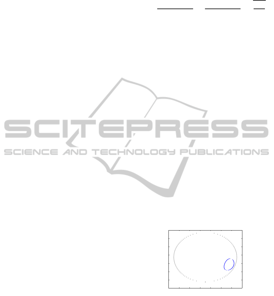
−200 0 200 400 600 800 1000 1200
−400
−200
0
200
400
600
800
1000
Figure 4: A test image generated by a paracatadioptric cam-
era.
Fig.4 shows a simulated paracatadioptric circle
image, where the larger conic is the projected con-
tour of parabolic mirror and the smaller curve is the
visible part of circle image. The projected contour
and the circle image are consisted of 100 points re-
spectively. Gaussian noise with mean 0 and standard
deviation σ ranging from 0 to 3 is directly added to
each of the points on the circle image. Because the
resolution of the image edge is lower than that of the
CalibratingFocalLengthforParacatadioptricCamerafromOneCircleImage
61

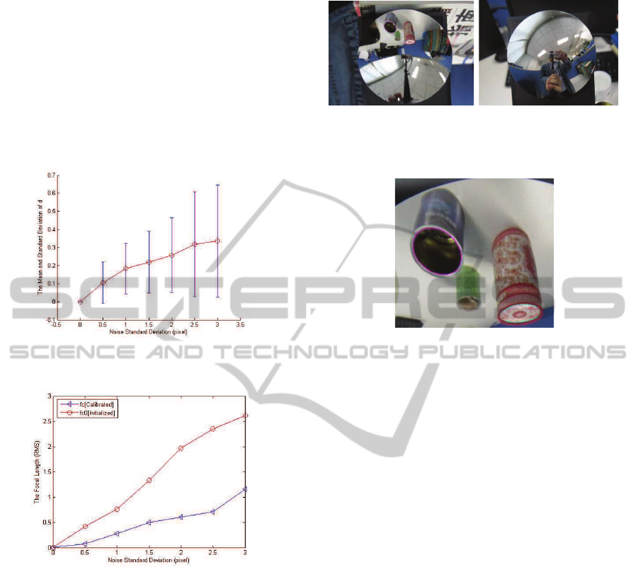
image center, we add noise with 2σ to the projected
contour of parabolic mirror. At each noise level, we
perform 100 independent trails respectively.
In the following, we use the algorithm proposed
in Section 4 to estimate the paracatadioptric circle im-
age. The mean and standard deviation of the algebraic
distance d from points to quartic curve (the circle im-
age) are shown in Fig.5. From Fig.5, it can be seen
that paracatadioptric circle can be estimated correctly,
which shows the validity of our fitting algorithm.
Figure 5: The mean and standard deviation of the distance
d from points to circle image.
Figure 6: The comparison result of the focal length.
Moreover, the focal length f
c
is computed through
the estimated paracatadioptric circle image and the
initialized principal point from Eq(19). Then, we
compare the computed focal length f
c
with the initial-
ized focal length f
c0
in Eq(15). Fig.6 gives the com-
parison result, which shows that the paracatadioptric
circle image can be estimated correctly.
5.2 Using Real Image Data
A real image of two cups is captured by a NIKON
COOLPIX990 with a hyperboloid mirror designed by
the Center for Machine Perception, Czech technical
University. The mirror parameter ξ = 0.966 that is
close to 1. Here, we approximately regard it as 1.
The image of cups is shown in Fig.7(a). Its size is
1080× 810 pixels.
(a) (b)
Figure 7: (a) A real image captured by a paracatadioptric
camera. (b) The test image.
Figure 8: The amplified result of estimated paracatadioptric
circle image.
The projected contour of mirror and circle
images (images of blue cup and red cup) are man-
ually extracted using the software in the website:
http//mail.isr.uc.pt/carloss/software/software.htm.
Next, applying the fitting algorithm proposed in
section 4, images of the two cups can be estimated.
To check the fitting result, we reproject the estimated
circle images to the original figure (Fig.7(a)). Fig.8
shows the amplified result, and we can see that the
circle images can be estimated correctly. In addition,
using the estimated circle images and the principal
point in Eq(15), the focal length is computed from
Eq(19). Then, the computed focal length and the
initialized principal point are used to rectify Fig.7(b).
Fig.9(a) and Fig.9(b) show the rectified results using
the images of two cups respectively. Intuitively, the
estimated intrinsic parameters can make those heavy
distorted lines become straight, i.e. the proposed
fitting method is very effective.
6 CONCLUSIONS
The projection of a circle under paracatadioptric cam-
era is a quartic curve. However, due to the partial
occlusion, it is impossible to directly estimate para-
catadioptric circle image using image points extract-
ing from the visible part. Consequently, camera pa-
rameters cannot be calibrated. In this paper, for the
case that aspect ratio is 1 and skew is 0, we study the
properties of paracatadioptric circle image and show
VISAPP2014-InternationalConferenceonComputerVisionTheoryandApplications
62

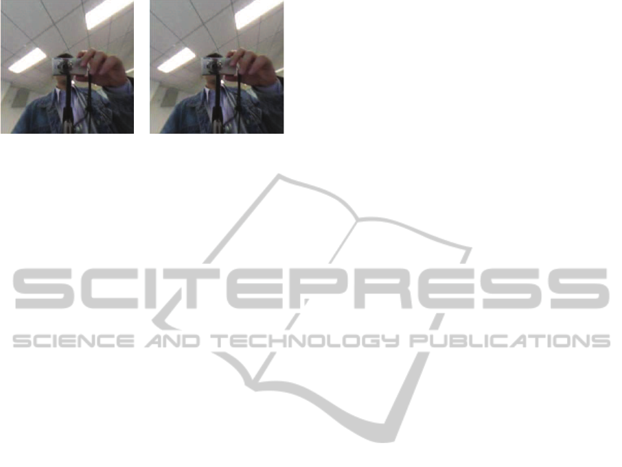
(a) (b)
Figure 9: (a) The rectified result through the image of blue
cup, (b) The rectified result through the image of red cup.
that the focal length can be calibrated from one circle
image. Firstly, we derive the necessary and sufficient
conditionsof paracatadioptric circle image. Secondly,
these conditions are used to limit the search space to
accurately estimate circle image. What’s more, we
show that the focal length can be computed from the
estimated circle image and the principal point that
is estimated from the projected contour of parabolic
mirror. Both the simulated and real data experiments
validate the effectiveness of our method. In our future
work, we continue to study the calibration method of
central catadioptric camera from circle images.
ACKNOWLEDGEMENTS
This work was supported by National Sci-
ence and Technology Support Projects of China
(No.2012BAH07B01).
REFERENCES
Alberto, R., E.Pedro, and Gines, G. (2002). A note on prin-
cipal point estimability. In Proc. International Conf.
on Pattern Recognition, pages 11–15. IEEE Press.
Aliaga, D. (2001). Accurate catadioptric calibration for
real-time pose estimation in room-size environments.
In Proc. International Conf. of Computer Vision,
pages 127–134. IEEE CS Press.
Baker, S. and Nayer, S. (1999). A theory of single-
viewpoint catadioptric image formation. Int. J. Com-
put. Vision, 35:175–196.
Barreto, J. and Araujo, H. (2002). Geometry properties of
central catadioptric line images. In Proc. European
Conf. of Computer Vision, pages 237–251.
Barreto, J. and Araujo, H. (2003). Paracatioptric camera
calibration using lines. In Proc. International Conf. of
Computer Vision. IEEE CS Press.
Barreto, J. and Araujo, H. (2005). Geometry properties of
central catadioptric line images and application in cal-
ibration. IEEE Trans. Pattern Anal. Machine Intell.,
27:1327–1333.
Barreto, J. and Araujo, H. (2006). Fitting conics to para-
catadioptric projection of lines. Computer Vision and
Image Understanding, 101:151–165.
Bastanlar, Y., Puig, L., Sturm, P., and Barreto, J. (2008).
Dlt-like calibration of central catadioptric cameras. In
Proc. Workshop on Omnidirectional Vision, Camera
Networks and Non-Classical Cameras.
Deng, X., Wu, F., and Wu, Y. (2007). An easy calibration
method for central catadioptric cameras. Acta Auto-
matica Sinica, 33:801–808.
Duan, F., Wu, F., Zhou, M., Deng, X., and Tian, Y. (2012).
Calibrating effective focal length for central catadiop-
tric cameras using one space line. Pattern Recognition
Letters, 33:646–653.
Duan, H. and Wu, Y. (2011a). Paracatadioptric camera
calibration using sphere images. In Proc. Interna-
tional Conf. on Image Processing, pages 649–652.
IEEE Press.
Duan, H. and Wu, Y. (2011b). Unified imaging of geo-
metric entities under catadioptric camera and camera
calibration. Journal of Computer-Aided Design and
Computer Graphics, 23:891–898.
Duan, H. and Wu, Y. (2012). A calibration method for
paracatadioptric camera from sphere images. Pattern
Recognition Letters, 33:677–684.
Geyer, C. and Daniilidis, K. (1999). Catadioptric camera
calibration. In Proc. International Conf. of Computer
Vision, pages 398–404. IEEE CS Press.
Geyer, C. and Daniilidis, K. (2001). Catadioptric projective
geometry. Int. J. Comput. Vision, 45:223–243.
Geyer, C. and Daniilidis, K. (2002). Paracatadioptric cam-
era calibration. IEEE Trans. Pattern Anal. Machine
Intell., 24:687–695.
Kang, S. (2000). Catadioptric self-calibration. In Proc.
IEEE Conf. on Computer Vision and Pattern Recog-
nition, volume 1, pages 201–207.
Scaramuzza, D., Martinelli, A., and Siegwart, R. (2006). A
flexible technique for accurate omnidirectional cam-
era calibration and structure from motion. In Proc.
International Conf. of Computer Vision, pages 45–52.
IEEE CS Press.
Sturm, P. and Barreto, J. (2008). General imaging geometry
for central catadioptric cameras. In Proc. European
Conf. of Computer Vision, pages 609–622.
Wu, F., Duan, F., Hu, Z., and Wu, Y. (2008). A new linear
algorithm for calibrating central catadioptric cameras.
Pattern Recognition, 41:3166–3172.
Wu, Y. and Hu, Z. (2005). Geometric invariants and ap-
plications under catadioptric camera model. In Proc.
International Conf. of Computer Vision, pages 1547–
1554. IEEE CS Press.
Wu, Y., Li, Y., and Hu, Z. (2006). Easy calibration for para-
catadioptric-like camera. In Proc. International Conf.
on Intelligent Robots and Systems, pages 5719–5724.
IEEE Press.
Ying, X. and Hu, Z. (2004). Catadioptric camera calibration
using geometric invariants. IEEE Trans. Pattern Anal.
Machine Intell., 26:1260–1271.
Ying, X. and Zha, H. (2008). Identical projective geomet-
ric properties of central catadioptric lines images and
sphere images with applications to calibration. Int. J.
Comput. Vision, 78:89–105.
CalibratingFocalLengthforParacatadioptricCamerafromOneCircleImage
63