Using Channel Representations in Regularization Terms

A Case Study on Image Diffusion

Christian Heinemann

, Freddie

Astr

, George Baravdish

, Kai Krajsek

, Michael Felsberg

and Hanno Scharr

IBG-2: Plant Sciences, Forschungszentrum J

ulich, 52425 J

ulich, Germany

Department of Electrical Engineering, Link

oping University, SE-581 83 Link

oping, Sweden

Department of Science and Technology, Link

oping University, SE-601 74 Norrk

oping, Sweden

Keywords:

Image Enhancement, Channel Representation, Channel Smoothing, Diffusion, Energy Minimization.

Abstract:

In this work we propose a novel non-linear diffusion ﬁltering approach for images based on their channel

representation. To derive the diffusion update scheme we formulate a novel energy functional using a soft-

histogram representation of image pixel neighborhoods obtained from the channel encoding. The resulting

Euler-Lagrange equation yields a non-linear robust diffusion scheme with additional weighting terms stem-

ming from the channel representation which steer the diffusion process. We apply this novel energy formula-

tion to image reconstruction problems, showing good performance in the presence of mixtures of Gaussian and

impulse-like noise, e.g. missing data. In denoising experiments of common scalar-valued images our approach

performs competitive compared to other diffusion schemes as well as state-of-the-art denoising methods for

the considered noise types.

1 INTRODUCTION

The channel representation (Granlund, 2000) is a

special, lossless soft-histogram, in contrast to other

histograms. Encoding a single value in a channel

representation, the value can be accurately recon-

structed. Using the channel representation allows for

simple outlier-removing smoothing, so called channel

smoothing (Felsberg et al., 2006), by essentially for

each pixel encoding the values of its local neighbor-

hood into a soft-histogram and assigning the decoded

value of the dominant mode to it, i.e. the sub-’bin’-

position of the maximum value in the soft-histogram.

This paper studies the nature and performance

of regularization terms penalizing the gradient of a

channel-smoothed signal. The rational behind this

is the observation, that in a robust diffusion scheme

(Perona and Malik, 1990), which can be derived from

a regularization term penalizing the gradient of a sig-

nal, the smoothing process is stopped or reduced at

edges, i.e. high gradient values. An outlier may erro-

neously be detected as edge and by this not smoothed

away. Not considering the outlier in the penalizing

term thus is expected to result in still high smoothing

strengths at outlier positions, reducing their visibility.

The natural test case for such a regularization is its

use without a data term, i.e. image diffusion not reg-

ularization. Further, as the robustness to outliers is of

interest, one natural application is image reconstruc-

tion in the presence of mixed noises. We use mixtures

of Gaussian and impulse-like noise.

We do not expect to derive the novel best denois-

ing scheme for gray value image reconstruction and

our experiments show that state-of-the-art denoising

schemes do a better job here. However, this addi-

tional robustiﬁcation by channel smoothing can eas-

ily be transferred to application domains, where diffu-

sion schemes are used in practice. Diffusion schemes

have been derived e.g. for color (Kimmel et al., 1998),

vector (Tschumperl

e and Deriche, 2005), or matrix-

valued data (Burgeth et al., 2007). They are applied

for regularization of DTMRI (Krajsek et al., 2008) or

high angular resolution diffusion imaging (HARDI)

data (Goh et al., 2011). Instead of a scalar-valued dif-

fusivities, tensorbased diffusion schemes use tensor-

valued diffusivities describing single or multiple ori-

entations in the image to drive the diffusion process

(Weickert, 1998; Scharr, 2006).

Crucial for the performance of non-linear diffu-

sion is an adaptation of the diffusivity, i.e. the local

smoothing strength, to image structure. Typically im-

age structure is measured as the Euclidean norm of

Heinemann C., Åström F., Baravdish G., Krajsek K., Felsberg M. and Scharr H..

Using Channel Representations in Regularization Terms - A Case Study on Image Diffusion.

DOI: 10.5220/0004667500480055

In Proceedings of the 9th International Conference on Computer Vision Theory and Applications (VISAPP-2014), pages 48-55

ISBN: 978-989-758-003-1

 2014 SCITEPRESS (Science and Technology Publications, Lda.)

the local image gradient. It is transformed into a dif-

fusivity by means of a edge-stopping function, assign-

ing small diffusivities to locations with high gradient

and vice versa. The exact choice of the edge-stopping

function has been shown to be equivalent to the choice

of error norm in robust statistics (Black et al., 1998)

and can be learned from image statistics (Zhu and

Mumford, 1997; Roth and Black, 2005).

If outliers are present in the data, e.g. as salt-and-

pepper noise, or dropouts, other reconstruction meth-

ods than diffusion are usually applied, able to remove

outliers completely, e.g. median ﬁltering (see e.g.

(Gonzalez and Woods, 2008)), or channel smoothing

(Felsberg et al., 2006) selecting the maximum mode

of the local value distribution. Channel smoothing

(CS) averages not only by applying a spatial window,

but also windows in the value domain. However, the

value domain window is not centered at the value of

the currently processed pixel, in contrast to bilateral

ﬁltering (Tomasi and Manduchi, 1998), but centered

at the maximum of the local value distribution. By

this, it removes clear outliers and interpolates from

neighbors. If Gaussian noise is present in the data,

also a part of the inliers are lost due to the value do-

main window and not considered in the value recon-

struction. Consequently the reconstructed gray value

is less efﬁciently denoised as if all inliers were con-

sidered.

1.1 Main Contributions

The core idea of this paper is to drive a non-linear

diffusion process using the CS result as image struc-

ture information. CS alone gives poor denoising re-

sults for medium to high Gaussian noise levels. In this

case, non-linear diffusion can yield higher signal-to-

noise-ratio (SNR) as it can average over all available

data. However, usual non-linear diffusion which is

driven by the local gradient stops at clear outliers, not

suppressing them. CS removes outliers while preserv-

ing edge location and roughly edge strength. Thus

driving a non-linear diffusion by CS allows to over-

smooth – not remove – outliers. We therefore expect

to gain SNR compared to plain CS when a consid-

erable amount of Gaussian noise is present and still

suppress outliers such that they are less visible in the

image. To derive the CS-based diffusion term, we de-

ﬁne an energy term penalizing the gradient of a chan-

nel encoded image.

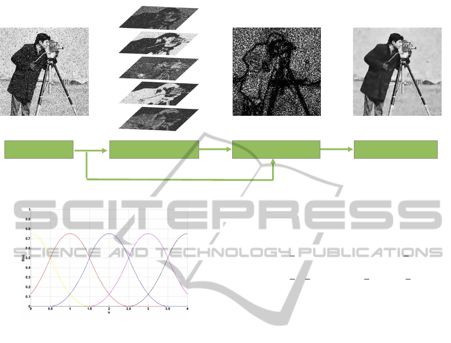
The schematic diffusion approach is illustrated in

Fig. 1. The noisy image is decomposed into its corre-

sponding channel representation. Within the channel

space we determine a local neighborhood which best

represents the data sample in the image space, thus we

guide a diffusion process such that Gaussian and im-

pulse noise is reduced which is indicated by the white

spots in the ”Filter & Update” step. Black indicates

no update, so important structure and edges in the im-

age are preserved.

Clearly, our diffusion process cannot remove out-

liers from data, but strongly smooth impulse-like

outliers. It is therefore well adapted to improve

the visual impression and preserving the structure

of reconstructed images, measured by SSIM (Wang

et al., 2004) in our experiments. Due to the mean-

preserving property of diffusion ﬁltering, bias-free

improvement of the reconstructed data values can

only be hoped for, when zero-mean noise is present.

2 BACKGROUND THEORY

In order to derive the novel non-linear channel-based

diffusion (NLCD) scheme in the subsequent section

we ﬁrst recall image diffusion derived from an energy

minimization, before the framework of channel repre-

sentation and channel smoothing is brieﬂy described.

2.1 Regularization and Image Diffusion

Let u(x, y) : Ω ⊂ R

→ R be a scalar valued image

deﬁned on a subset of R

. The variational approach

to image regularization or image diffusion

is to con-

sider an energy functional of the form

E(u) =

Ω

(u − u

)

dxdy + λR(u) , (1)

where R(u) is a regularization term, λ ∈ R, λ > 0 con-

trols the inﬂuence of the regularization and u

is the

observed image. In particular let R(u) be selected as

R(u) =

Ω

|∇u|

dxdy , (2)

where the gradient operator is deﬁned as ∇ =



∂

, ∂



and

denotes the Euclidean norm. Then

the functional E(u) deﬁnes linear image regulariza-

tion: To minimize E(u) one can compute the varia-

tional derivative and by assuming Neumann bound-

ary conditions

∇u, n

= 0 for a boundary element n

Image regularization and image diffusion are closely

related. Image regularization is a boundary value problem,

equivalent to heat diffusion with source terms in physics.

Image diffusion is equivalent to heat diffusion without

sources, formulated as initial value problem, starting with

the measured, noisy image. In both cases, the regulariza-

tion term deﬁnes the smoothing process leading to noise

suppression. For simplicity, we call this process diffusion in

both cases, as usual in physics. For details of the very close

relation between regularization and diffusion see (Scherzer

and Weickert, 1998).

UsingChannelRepresentationsinRegularizationTerms-ACaseStudyonImageDiffusion

Noisy image Channel encode Denoised imageFilter & Update

Figure 1: Overview of proposed method. Contrast is increased in ”Filter & Update” for a better visualization.

Figure 2: Example for equidistantly distributed B-Spline

basis functions. Five channels are used here.

of ∂Ω, we obtain the Euler-Lagrange (EL) equation

described by the PDE



u − u

− λ∆u = 0

∇u, n

= 0.

(3)

The corresponding linear diffusion without data term

reads



∂

u = ∆u

∇u, n

= 0.

(4)

2.2 Channel Representation

This section introduces channel representations as an

approximative density estimator as described in (Fels-

berg et al., 2006). Channel representations are ba-

sically soft-histograms, i.e., histograms where sam-

ples are not exclusively pooled to the closest bin cen-

ter, but to several bins with a weight depending on

the distance to the respective bin center. The ’bins’

are called ’channels’. The binning operator or den-

sity mapping function is called a basis function, B(u),

and is usually non-negative (as densities are non-

negative), has compact support and is smooth (for sta-

bility reasons). The measure induced by the mapping

to channel representations should be position inde-

pendent in order to avoid an unwanted bias. In this

paper, quadratic B-splines are used as basis functions:

B(u) =











− u

0 ≤ |u| ≤



− |u|



< |u| ≤

0 Otherwise.

(5)

Without loss of generality we assume that u(x) ∈

[0, N − 1] before the signal can be encoded into N

channels. Otherwise we linearly transform u to that

interval. Figure 2 depicts the basis functions in the

case of 5 channels. Let c ∈ R

, N > 0, be an equidis-

tantly distributed grid over the image range of u. We

call c = (c

, . .. , c

)

channel center vector. Then

we obtain the quadratic B-Spline channel representa-

tion B

= B(u(x, y) − c

) where B = (B

, . .. , B

), i =

1, . .. , N is called channel vector.

In channel smoothing (Felsberg et al., 2006) the

channel vectors are spatially averaged using a Gaus-

sian kernel w resulting in

(x, y) = w ∗ B

(x, y). (6)

Reconstructing a value u from the channel represen-

tation can be done using a linear combination of all

channel vector components yielding a linear decod-

ing. To obtain a robust decoding scheme only a

subset of the channel components is used (Felsberg

et al., 2006). In this work a window of size 3 around

the maximum mode location of the channel vector is

computed i.e.

l = argmax

∑

k+1

i=k−1

(x, y) (7)

with k = 2, . . . , N − 1. Then the robust decod-

ing scheme, also used in the framework of channel

VISAPP2014-InternationalConferenceonComputerVisionTheoryandApplications

smoothing (Felsberg et al., 2006), reads

ˆu(x, y) =

l+1

∑

i=l−1

(x, y) . (8)

where we assume that the coeffcients

(x, y) sum up

to one, if not, we normalize them to do so. Note that

the choice of l in (7) depends on continuously differ-

entiable basis functions such that the local maxima

are continuous functions of the input values. The or-

der of local maxima depends on the clusters of the

inputs, but this is desirable since this reﬂects e.g. the

non-stationarity across edges.

3 IMAGE DIFFUSION WITH THE

CHANNEL FRAMEWORK

In this section we introduce an energy functional

combining the framework of diffusion ﬁltering and

channel representation in order to ﬁrst derive linear

channel-based diffusion (LCD) before extending it to

the non-linear case (NLCD).

3.1 Introducing Channel

Representation to Linear Image

Diffusion

In order to enable diffusion methods to oversmooth

impulse noise, we deﬁne the regularization term R(u)

using the channel representation as described in the

previous section. We encode u into the channel space

using (8) thus leading to the regularization term

R(u) =

Ω

|∇

l+1

∑

i=l−1

(x, y)|

dxdy , (9)

where l is deﬁned in (7) and

B are the smoothed chan-

nel weights as in (6). With notational abuse, to sim-

plify notation, we deﬁne in the subsequent derivation

l+1

∑

i=l−1

(x, y) = c

B , (10)

where the 3-box windowing is implicitly included in

B(u). The integrand of R(u) can then be written in

vector-matrix notation as |∇(c

B)|

which yields

R(u) =

Ω



(∂

B)(∂

+ (∂

B)(∂



c dxdy .

(11)

To ﬁnd the EL-equation of (11) we compute the vari-

ational derivative, denoted as R

v =

∂R(u+εv)

∂ε



ε=0

, in

the direction of v with respect to u where v ∈ C

(Ω)

is a non-zero testfunction. We split the integral (11)

into two integrals calculating the x- and y-component

separately and get

v =

∂

∂ε



Ω

(u + εv)

· (∂

u + ε∂

c dxdy



ε=0

Ω



∂

∂ε

(u + εv)



ε=0



c(∂

+ 2c



(u)

∂

u∂



c dxdy

Ω



(u)



c(∂

v dxdy

− 2

Ω

∂



(u)

c∂



v dxdy .

The same holds for the y-component. For the last

equation we applied Green’s formula and Neumann

boundary conditions to get rid of the ∂

v term which

cannot be determined. To further simplify nota-

tion let S(u) =

(u)

. Using the deﬁnition

of divergence and the equality div(c

S(u)c ∇u) =

(u)c∇u (∇u)

S(u)c ∆u the variation of the en-

ergy in the direction of v can be formulated as

v = −



div



S(u)c ∇u



+ c

S(u)c ∆u



v .

With the derived functional derivative we are able to

obtain the PDE



∂

u = div(c

S(u)c ∇u) + c

S(u)c ∆u

∇u, n

= 0,

(12)

where λ > 0 is a constant. The matrix S(u) is a sym-

metric matrix with entries as a block of size three

centered around the main diagonal (cmp. Figure 3a).

Since S(u) is the outer product of the vector

, it is

positive semi deﬁnite. The scalar value c

S(u)c acts as

a weight and we obtain a coefﬁcient with large entires

in homogeneous areas as the box decoding includes

almost all relevant values. At edges the coefﬁcient

has low entries. At outlier positions the coefﬁcient is

still large (cmp. Figure 3b).

We observe that the right hand side of (12), top,

consists of two terms, where the left one has the usual

form of non-linear diffusion with spatial varying dif-

fusivity c

S(u)c, and the right one the form of a dif-

fusion term ignoring the spatial variation of c

S(u)c.

For linear decoding channel smoothing breaks down

to simple local averaging of u and c

S(u)c ≡ 1, inde-

pendent of the variance of w (cmp. (6)), and (12) be-

comes plain linear diffusion (4). Using robust decod-

ing c

S(u)c becomes a spatially varying function and

(12) a non-linear diffusion with reduced diffusivity at

edges and high diffusivity in homogenous regions as

well as at outlier positions (cmp. Figure 3b).

UsingChannelRepresentationsinRegularizationTerms-ACaseStudyonImageDiffusion

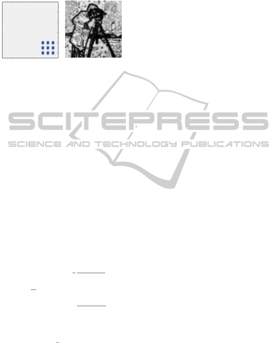
0 2 4 6 8 10

a) b)

Figure 3: a) Typical structure of S(u) for a certain spatial

position. The size of the matrix is equal to the number of

channels. In this example 11 channels are used and non-

zero entries are centered around channel 9. b) Structure of

S(u)c for the cameraman image and a Gaussian kernel w

with standard deviation 3. Black indicates low and white

high values close to 1.

3.2 Introducing Channel

Representation to Non-linear Image

Diffusion

Here the LCD will be extended to its non-linear pen-

dant including a convex potential function Φ. The

motivation is to further control the ﬁltering to pre-

serve ﬁne image details, similarly to the approach by

Perona and Malik (Perona and Malik, 1990). Includ-

ing a potential function allows to suppress outliers

further as they will not appear in the structure esti-

mation.

Let the regularization term be deﬁned as

R(u) =

Ω

Φ(|∇(c

B(u))|)dxdy , (13)

where c

B(u) is the channel smoothed version of the

image u as deﬁned in (8). By computing the varia-

tional derivative R

v in a similar way as presented in

the previous section we obtain

v =

Ω

(|∇(c

B(u))|)

|∇(c

B(u))|

∂

∂ε



|∇(c

B(u + εv))|



ε=0

dxdy.

(14)

Using the short notation Ψ =

(|∇(c

B(u))|)

|∇(c

B(u))|

and the

derivation from the previous section, the EL-equation

reads











∂

u = λ



Ψ div(c

S(u)c)∇u

S(u)c div(Ψ∇u)



∇u, n

= 0,

(15)

where λ > 0 and S(u) =

(u)

as before.

The two right hand terms of (15) both implement non-

linear diffusion weighted by an additional factor. In

the ﬁrst term the diffusivity stemms from the channel

representation and the usual edge stopping function

Ψ acts as additional weight. In the second term the

roles of Ψ and c

S(u)c are exchanged. Furthermore,

Ψ is deﬁned on the channel smoothed image c

B(u),

so outliers are not present in the structure estimation

of Ψ and will be smoothed strongly.

4 EXPERIMENTS

In this section we evaluate the proposed linear chan-

nel diffusion (LCD) and the non-linear channel diffu-

sion (NLCD) for different grey-scale images. Stan-

dard images as ”Cameraman” are used as well as

images from the Berkeley image database (Martin

et al., 2001) commonly used for segmentation pur-

poses. Since we are interested in investigating the

case of a mixture of noise models we corrupt the im-

ages with Gaussian noise as well as impulse noise.

Here we consider the presence of 5% impulse noise

and vary the standard deviation of Gaussian noise

σ ∈

{

5, 10, 15,20, 30, 40, 50

}

4.1 Setup of Evaluation

The aim of the evaluation is to compare the pro-

posed LCD and NLCD schemes especially to dif-

fusion schemes and channel smoothing as we intro-

duced an extension of these methods. Current state-

of-the-art denoising methods are included as well.

We compare to linear diffusion (LD) and non-linear

diffusion (NLD) as introduced by Perona-Malik (Per-

ona and Malik, 1990). Furthermore, we consider the

tensor-driven anisotropic diffusion scheme (AD) (We-

ickert, 1998). Besides channel smoothing (CS) (Fels-

berg et al., 2006), median ﬁltering (MF) is included

as a method well suited for impulse noise. Further

BM3D (Dabov et al., 2006) is regarded, currently

one of the best methods for ﬁltering Gaussian noise.

It considers both a non-linear threshold operation as

well as a linear Wiener ﬁlter approach to a stack of

patches which locally describe the same image region.

Finally, two implementations of non-local means are

regarded. We compared to the original, pixel based

implementation (Buades and Coll, 2005) as well as to

the the patch based variant (Buades et al., 2011).

All methods have been optimized with respect to

their parameters. We optimized LCD and NLCD with

respect to the number of channels and the edge pa-

rameter α in the edge stopping function Ψ, which

VISAPP2014-InternationalConferenceonComputerVisionTheoryandApplications

234

2.5

3.5

linear diffusion

non−linear diffusion

anisotropic diffusion

channel smoothing

linear channel diffusion

non−linear channel diffusion

0 5 10

Median filter

BM3D

NLM patchbased

10 20 30 40 50

0.6

0.7

0.8

0.9

SSIM

Noise level

Cameraman

10 20 30 40 50

0.5

0.6

0.7

0.8

0.9

SSIM

Noise level

Skyline

10 20 30 40 50

0.8

0.85

0.9

0.95

SSIM

Noise level

Hawk

10 20 30 40 50

0.8

0.85

0.9

0.95

SSIM

Noise level

Bird

10 20 30 40 50

0.6

0.7

0.8

0.9

SSIM

Noise level

Rollercoaster

10 20 30 40 50

0.7

0.75

0.8

0.85

0.9

0.95

SSIM

Noise level

House

10 20 30 40 50

0.7

0.8

0.9

SSIM

Noise level

Lena

10 20 30 40 50

0.7

0.8

0.9

SSIM

Noise level

Boat&House

10 20 30 40 50

0.6

0.7

0.8

0.9

SSIM

Noise level

Lighthouse

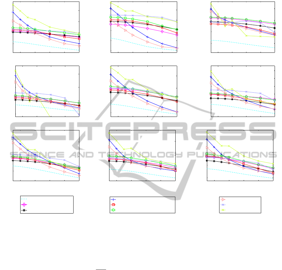
Figure 4: Quantitative denoising results of the images Skyline (69007), Hawk (42040), Bird (197027), Rollercoaster (235098),

Boat &House (140088) and Lighthouse (228076) from the Berkeley image database (Martin et al., 2001) and standard test

images (Cameraman, House, Lena). The numeric name is the same as in the database. Used methods are linear diffusion,

NLD (Perona and Malik, 1990), AD (Weickert, 1998), CS (Felsberg et al., 2006), the novel LCD, the novel NLCD, MF

(Gonzalez and Woods, 2008), BM3D (Dabov et al., 2006) and NLM (Buades et al., 2011). SSIM versus different Gaussian

noise levels is plotted. For details see text. Best viewed in color

has been chosen as Ψ(|∇u|) = (1 +

|∇u|

)

−1

. Fur-

thermore, the size of the median ﬁlter was optimized.

For the channel smoothing (CS) we use a box decod-

ing scheme, optimize the number of channels, and

optimize the variance of the Gaussian ﬁlter used for

smoothing in each channel. In AD, the mapping of the

structure tensor eigenvalues to diffusivities is done us-

ing the same edge stopping function as for NLD. The

parameter α is also optimized.

We implement our diffusions in a standard Euler

forward scheme and use ﬁnite differences to approx-

imate the image derivatives for every spatial position

in the image. For each method and parameter opti-

mization we let the ﬁltering continue until the maxi-

mum of the structure similarity index (SSIM) (Wang

et al., 2004) has been reached.

4.2 Results

In Figure 4 we show the best obtained SSIM value

for each image and considered noise level. The pixel

based NLM variant (Buades and Coll, 2005) has

SSIM values between 0.3 and 0.5 for all images as

it poorly reduces impulse noise. To focus on higher

SSIM values we do not show values for pixel NLM.

Generally, best denoising results are obtained by

the patch version of the non-local means, especially

for low gaussian noise levels. BM3D also gains high

SSIM. For low Gaussian noise CS shows good results

as well. This was expected as channel smoothing, as

well as median ﬁltering, are well suited methods for

removing clear outliers. The NLCD gives quite high

SSIM for higher Gaussian noise levels.

For few special cases we observe that NLCD per-

UsingChannelRepresentationsinRegularizationTerms-ACaseStudyonImageDiffusion

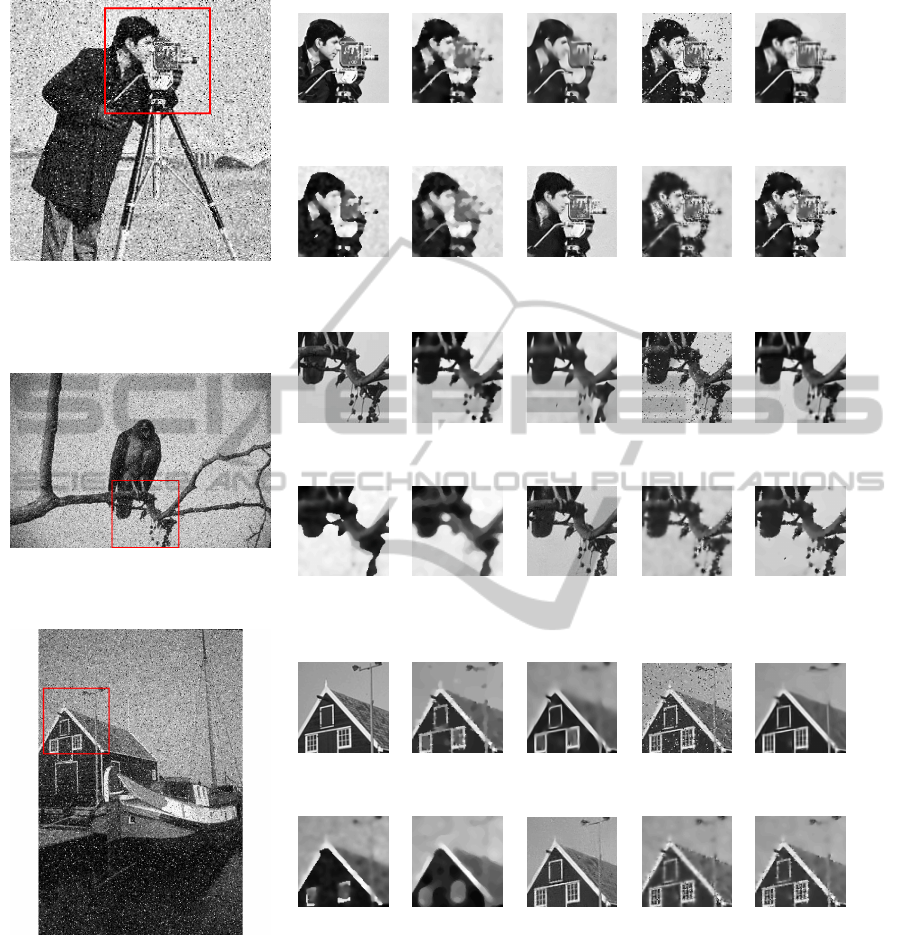
Cameraman

Initial noise = 0.2692

Original NLD AD NLM pixel BM3D

0.6874 0.6858 0.3753 0.7145

CS MF NLM patch LCD NLCD

0.6606 0.6393 0.7408 0.6871 0.7126

Hawk

Initial noise = 0.1460

Original NLD AD NLM pixel BM3D

0.8989 0.8832 0.2822 0.8963

CS MF NLM patch LCD NLCD

0.8694 0.8632 0.8329 0.8705 0.9028

Boat&House

Initial noise = 0.1687

Original NLD AD NLM pixel BM3D

0.7511 0.7380 0.2964 0.7624

CS MF NLM patch LCD NLCD

0.7269 0.7242 0.7798 0.7481 0.7665

Figure 5: Visualization of certain parts of different images (Cameraman, Hawk, Boat&House) of noise level σ = 30. A visual

comparison is done between the introduced methods.

forms best, even better than the state-of-the-art de-

noising methods BM3D and NLM, which is unex-

pected, see e.g. result for the hawk image. In all cases

NLCD is comparable and most times better than the

other diffusion-based methods, especially well e.g.

in the skyline image or the cameraman. As soon as

Gaussian noise of around σ = 15 or σ = 20 has been

added to the image the NLCD also ouperforms CS.

The aim of this work was not to construct the best

denoising algorithm but to combine the advantages of

channel smoothing and diffusion based schemes. The

NLCD outperforms in all cases CS if a medium or

high amount of Gaussian noise is present and it out-

performs in most cases NLD and AD for all noise lev-

els. In some cases NLCD even shows competitive re-

sults compared to state-of-the-art denoising methods.

In Figure 5 a visualization of certain image close

ups can be seen. The CS and MF show a comic like

VISAPP2014-InternationalConferenceonComputerVisionTheoryandApplications

behavior, maintaining the main edges well but details

are lost as can be seen in the face or the camera. The

pixel based NLM cannot handle the impulse noise at

all. Better preservation of details is achieved using

AD or NLD. Good results show the patch based NLM

and BM3D. However, for patch NLM the image still

shows some Guassian noise and for BM3D still some

details are lost. The proposed LCD show an improve-

ment compared to CS and MF, but due to its linear

form the edges are smeered. Visually, better results

compared to CS and diffusion methods are obtained

with NLCD. It keeps the details and it is able to han-

dle impulse noise as well as Gaussian noise.

5 CONCLUSIONS

For the aim of ﬁltering noisy images a new linear and

a new non-linear diffusion scheme has been presented

using advantages of channel representations. For this

purpose we derived an iterative ﬁltering scheme by

minimizing a corresponding energy functional. In-

cluding the channel framework leads to a robust ﬁl-

tering well suited for images corrupted with Gaus-

sian as well as impulse noise. We analysed the de-

noising behaviour of the proposed method on com-

monly used scalar valued images and compared the

methods to similar as well as state of the art meth-

ods. It turned out that the new method outperforms

the other diffusion-based methods if impulse noise

and a medium or high amount of Gaussian noise are

present. In some cases it even outperforms state-of-

the-art denoising methods. In future investigations,

application of the novel NLCD scheme to DTMRI

and HARDI data may be of interest.

ACKNOWLEDGEMENTS

This research has been in part supported by the

Swedish Research Council through a grant for the

project Visualization-adaptive Iterative Denoising of

Images and has received in part funding from the Eu-

ropean Communitys Seventh Framework Programme

FP7/2007-2013 Challenge 2 Cognitive Systems, In-

teraction, Robotics under grant agreement No 247947

GARNICS.

REFERENCES

Black, M., Sapiro, G., Marimont, D., and Heeger, D.

(1998). Robust anisotropic diffusion. TIP, pages 421–

432.

Buades, A. and Coll, B. (2005). A non-local algorithm for

image denoising. In CVPR, pages 60–65.

Buades, A., Coll, B., and Morel, J.-M. (2011). Non-Local

Means Denoising. Image Processing On Line, 2011.

Burgeth, B., Didas, S., Florack, L., and Weickert, J. (2007).

A generic approach to diffusion ﬁltering of matrix-

ﬁelds. Computing, 81:179–197.

Dabov, K., Foi, A., Katkovnik, V., and Egiazarian, K.

(2006). Image denoising with block-matching and 3d

ﬁltering. In Electronic Imaging’06, Proc. SPIE 6064.

Felsberg, M., Forss

en, P.-E., and Scharr, H. (2006). Channel

smoothing: Efﬁcient robust smoothing of low-level

signal features. PAMI, 28(2):209–222.

Goh, A., Lenglet, C., Thompson, P. M., and Vidal, R.

(2011). A nonparametric riemannian framework for

processing high angular resolution diffusion images

and its applications to odf-based morphometry. Neu-

roImage, 56(3):1181 – 1201.

Gonzalez, R. C. and Woods, R. E. (2008). Digital Image

Processing - 3d edition. Pearson International Edition.

Granlund, G. H. (2000). An associative perception-action

structure using a localized space variant information

representation. In Proceedings of AFPAC.

Kimmel, R., Malladi, R., and Sochen, N. A. (1998). Image

processing via the Beltrami operator. In ACCV LNCS,

pages 574–581.

Krajsek, K., Menzel, M., Zwanger, M., and Scharr, H.

(2008). Riemannian anisotropic diffusion for tensor

valued images. In ECCV, LNCS, pages 326–339.

Martin, D., Fowlkes, C., Tal, D., and Malik, J. (2001). A

database of human segmented natural images and its

application to evaluating segmentation algorithms and

measuring ecological statistics. In ICCV. 416–423.

Perona, P. and Malik, J. (1990). Scale-space and edge detec-

tion using anisotropic diffusion. PAMI, 12:629–639.

Roth, S. and Black, M. J. (2005). Fields of experts: A

framework for learning image priors. In CVPR. 860–

867.

Scharr, H. (2006). Diffusion-like reconstruction schemes

from linear data models. In Pattern Recognition

LNCS, volume 4174, pages 51–60, Berlin. Springer.

Scherzer, O. and Weickert, J. (1998). Relations between

regularization and diffusion ﬁltering. Journal of Math-

ematical Imaging and Vision, 12:43–63.

Tomasi, C. and Manduchi, R. (1998). Bilateral ﬁltering for

gray and color images. In ICCV, pages 839–846.

Tschumperl

e, D. and Deriche, R. (2005). Vector-valued im-

age regularization with pdes: A common framework

for different applications. PAMI, 27(4):506–517.

Wang, Z., Bovik, A., Sheikh, H., and Simoncelli, E. (2004).

Image quality assessment: from error visibility to

structural similarity. IEEE TIP, 13(4):600 –612.

Weickert, J. (1998). Anisotropic Diffusion In Image Pro-

cessing. ECMI Series, Teubner-Verlag, Stuttgart.

Zhu, S. C. and Mumford, D. (1997). Prior learning and

gibbs reaction-diffusion. PAMI, 19:1236–1250.

UsingChannelRepresentationsinRegularizationTerms-ACaseStudyonImageDiffusion