
Advanced Learning Techniques for Chemometric Modelling
Carlos Cernuda
1,2
, Edwin Lughofer
1,2
and Erich Peter Klement
1,2
1
Institute of Knowledge-Based Mathematical Systems, JKU Johannes Kepler University Linz,
Altenbergerstrasse 66, Linz, Austria
2
FLLL Fuzzy Logic Lab Linz, Softwarepark 21, Hagenberg im Muhlkreis, Austria
1 ABSTRACT
The European chemical industry is the world leader
in its field. 8 out of the 15 largest chemical
companies are EU based. Furthermore, 29 % of the
worldwide chemical sales originate from the EU.
These industries face future challenges such as rising
costs and scarcity of raw materials, an increase in
the price of energy, and an intensified
competition from Asian countries.
Process Analytical Chemistry represents one of
the most significant developments in chemical and
process engineering over the past decade. Chemical
information is of increasing importance in today's
chemical industry. It is required for efficient process
development, scale-up and production. It is used to
assure product quality and compliance with
regulations that govern chemical production
processes.
If reliable analytical information on the chemical
process under investigation is available, adjustments
and actions can be undertaken immediately in order
to assure maximum yield and product quality
while minimizing energy consumption and waste
production. As a consequence, chemical information
has a direct impact on the productivity and thus
competitiveness, and on the environmental issues of
the respective industries.
Chemometrics is the application of mathematical
or statistical methods to chemical data. The
International Chemometrics Society (ICS) offers the
following definition:
“Chemometrics is the science of relating
measurements made on a chemical system or
process to the state of the system via application of
mathematical or statistical methods”.
Chemometric research spans a wide area of
different methods which can be applied in
chemistry. There are techniques for collecting good
data (optimization of experimental parameters,
design of experiments, calibration, signal
processing) and for getting information from these
data (statistics, pattern recognition, modeling,
structure-property-relationship estimations).
In this extense list of tasks, we are focused on
calibration. Calibration consists on stablishing
relationships, i.e. chemometric models, between
some instrumental response and chemical
concentrations. The usual instrumental responses
come from the use of spectrometers, because they
allow us to get a lot of on-line cheap data in a non-
destructive way. There are two types of calibration,
univariate or multivariate calibration, depending on
the use of only a single predictor variable or several
ones.
The current instalations provide us with
thousands of variables and thousands of samples,
thus more and more new sophisticated techniques,
which are capable to handle and take advantage of
this tsunami of data, are required.
Our goal is to provide the analytical chemistry
community with modern and sophisticated tools in
order to overcome the incoming future challenges.
2 STAGE OF THE RESEARCH
The title for the PhD thesis is “Advanced Learning
Techniques for Chemometric Modelling”. The
research is carried out as part of the research K-
project called “Process Analytical Chemistry – Data
Acquisition and Data-processing” (PAC).
The K-project PAC bundles industrial and
academic research in Process Analytics. The PAC
consortium intends to develop and implement
technologies which allow for a direct and remote
acquisition of chemical information on continuous
and batch processes which are currently run at the
production sites of the industrial partners.
The scope of the research program comprises:
Development and integration of novel
detection principles for the measurement of
data representing the chemical properties of the
involved substances. The acquisition is
19
Cernuda C., Lughofer E. and Klement E. (2013).
Advanced Learning Techniques for Chemometric Modelling.
In Doctoral Consortium, pages 19-28
Copyright
c
SCITEPRESS

performed directly from the running batch and
continuous processes (Data Acquisition).
Development and application of novel
approaches for turning the measured data into
valid information on the ongoing chemical
processes (Data Processing).
The project is organised in form of 6 sub-
projects, with 4 of them being executed by the
scientific partners in close colloboration with the
company partners (4 multifirm-projects). The other 2
sub-projects are called strategic projects and their
scope is mainly scientific:
Multifirm-Project MP1: Quantification of
Process Gases.
Multifirm-Project MP2: Quantifying and
Predicting Parameters of Liquids in BATCH
Processes.
Multifirm-Project MP3: Quantification of
Parameters and Detection of Anomalies
and critical Parameters in Liquids within
continuous Processes.
Multifirm-Project MP4: Monitoring the
Production of Viscose Fibres.
Strategic Project SP1: Advanced Chemometric
Modelling.
Strategic Project SP2: QCL-WAGS - Sensor
Systems (Quantum Cascade Lasers and Wave
Guide - Structures).
Our research work is maily related to Strategic
Project 1, with some punctual collaboration in the
Multifirm projects 2, 3 and 4. Therefore it is directly
related with the field of Chemometrics.
The project duration is four years, finishing in
September 2014. Thus 75% of the work is already
done in this moment.
3 OUTLINE OF OBJECTIVES
The intention of our research is to provide the
chemometric community with a bunch of new
advanced techniques, some totally new and some
adapted from other fields, so that they overcome the
traditional State-of-Art linear methods.
Our intention is to try to cover all aspects of the
chemometric modelling process, from preprocessing
to validation and posterior adaptation, in more or
less depth. We will describe the objectives, ordering
them in terms of the different steps of the modelling:
Preprocessing: explore several new off-line
outlier detection methods based on the use of
different distance measures, and also on the
information provided by the application of
projection methods which permit a better
understanding of the data properties.
Dimensionality reduction / variable selection:
use of metaheuristic optimization algorithms,
like ant colony optimization (ACO) or particle
swarm optimization (PSO) to look for the
variables that explain best the relationships
underlying in our calibration data. For the same
purpose, also the use of genetic algorithms
(GA), with specifically designed genetic
operators, will be explored. Moreover, hybrid
approaches combining the diverse optimization
characteristics of the previous algorithms will
be employed. Furthermore, traditional forward
and backward selection algorithms do not take
into account the problem specific information.
Therefore we will propose algorithms, like
forward selection bands (FSB), which take the
advantages of the physical/chemical knowledge
of the chemical process in order to make better
selections.
Off-line batch modelling: use of flexible fuzzy
inference systems, as a non-linear alternative to
the conventional linear methods commonly
employed in chemometrics nowadays.
Incorporation of external independent
information decoupled from the spectroscopy
data, coming from sensors. Develop techniques
that can handle repeated measurements, in a
more advanced way than the classical
averaging approach, by means of procedures
similar to bagging and ensembling.
Robustness analysis: definition of different
types of confidence intervals and error bars in
order to estimate the uncertainty present in the
predictions of our off-line models.
On-line modelling: development incremental
versions of the outlier detection methods, in
order to handle possible incoming outliers in a
continuous process. Try to perform incremental
adaptations of the S-o-A linear modelling
techniques when possible. Use of incremental
flexible fuzzy inference systems, exploiting all
its capabilities, e.g. rules merging, rules
pruning, forgetting strategies. Use of retraining
strategies based on sliding windows, with
many alternatives on how to create, update and
handle the window, as an alternative to
incremental approaches. Pros and cons of both
options will be discussed.
IJCCI2013-DoctoralConsortium
20

Validation techniques: specific validation
techniques will be used in specific cases, for
instance in the presence of repeated
measurements or when using extra independent
sources of information.
Cost optimization: not present usually in
research on chemometrics, but unavoidable in
real world applications. Active learning (AL)
strategies, both decremental and incremental,
will be developed.
Apart from being an advanced manual, full of new
options for the chemometricians, we pretend to
motivate the search of innovative techniques, as well
as to look what researchers from other fields are
doing, in order to be more open minded and
receptive. This would lead as towards a successful
self-adaptation to the new times that are coming.
4 RESEARCH PROBLEM
Due to the ever-increasing production of complex
data by a large variety of analytical technologies,
chemometric data analysis and data mining have
become crucial tools in modern science. This
increase in popularity of chemometrics has boosted
the awareness of its potential in the era in which data
tsunamis rule the scientific world. However, it is
evident that serious shortcomings have so far
hampered the full exploitation of the chemometric
potential. First, there is a lack of an underlying
generic strategy for the data analysis workflow. This
means that in practice each different data set
requires its own research project to define the
optimal pre-processing and data analysis settings to
cope with its own peculiarities originating from
different sources. Second, the usual workhorses such
as principal component analysis (PCA), while
designed to cope with large multivariate data, are not
suitable anymore for the complex mega-variate
and/or multiway data originating from, e.g.,
comprehensive profiling techniques.
Advanced preprocessing techniques as well as
robust and accurate non-linear complex models are
necessary to extract all the knowledge contained in
the data and fulfill the companies’ requirements
nowadays, in this global highly competitive
industrial world.
The incoming technical advances in data
adquisition permit us say that our entire world can
be storaged into data. Therefore, we have the
challenge and the oportunity of understanding the
world by means of adequate data mining techniques.
Everything is there, but we need the tools to see it.
5 STATE OF THE ART
The simplest regression method, multiple linear
regression (MLR), presents several well-known
disadvantages when applied to datasets where the
variables are highly correlated
The abundance of response variables relative to
the number of available samples which leads to
an undetermined situation.
The possibility of collinearity of the response
variables, which leads to unstable matrix
inversions and unstable regression results.
These problems can be dealt by means of other kinds
of regression, like principal components regression
(PCR) (Jolliffe, 2002), partial least squares (PLS)
regression (Haenlein and Kaplan, 2004), Ridge
Regression introducing a penalty term (Cernuda et
al., 2011), etc. In this sense, these approaches
enjoyed a great attraction in the field of
chemometric modeling resp. extracting models from
spectral data in general, see for instance (Reeves and
Delwiche, 2003; Vaira et al., 1999; Shao et al.,
2010) or (Miller, 2009).
In the following, we briefly summarize these
methods:
Principal components analysis (PCA) finds
combination of variables that describe major
trends in the data in an unsupervised manner.
The trends are characterized by those directions
along which the data has the maximal variance.
PCA performs a rotation of the coordinate
system using a singular value decomposition of
the covariance matrix (Jolliffe, 2002) such that
the axes of the new system are exactly lying in
these directions. The first principal component
with largest eigenvalue is expected to be the
most important rotated axis, the second
component with the second largest eigenvalue
the second most one, etc. According to this
order, components with the most significant
contributions are selected; where the remaining
ones contribute quite little to the full eigen-
space (the sum of their eigenvalues is low).
Regression is then conducted using the
selected components as inputs and the original
target as output variable.
Partial least squares regression (PLSR) is
related to both, PCR and MLR, and can be
thought of as stated in between them. The
former finds factors that capture the greatest
AdvancedLearningTechniquesforChemometricModelling
21

amount of variance in the predictor variables
while the latter seeks to find a single factor that
best correlates predictor variables with
predicted variables. PLS attempts to find
factors which both capture variance and
achieve correlation by means of projecting not
only the predictor variables (like PCA), but
also the predicted ones, to new spaces so that
the relationship between successive pairs of
scores is as strong as possible.
Locally weighted regression (LWR) (Cleveland
and Devlin, 1988) is a procedure for fitting a
regression surface to data through multivariate
smoothing: the dependent variable is smoothed
as a function of the independent variables in a
moving fashion, analogs to how a moving
average is computed for a time series.
Regression Trees (RegTree) (Cernuda et al.,
2011) use the tree to represent the recursive
partition of the input space in small local parts
thus bringing in some non-linearity. Each of
the terminal nodes, or leaves, of the tree
represents a cell of the partition, and has
attached to it a simple model which applies in
that cell only.
Stepwise Regression (StepwiseReg) (Draper
and Smith, 1998) removes and adds variables
to the regression model for the purpose of
identifying a useful subset of the predictors.
The choice of predictive variables is carried out
by an automatic procedure, based on a
sequence of F-tests.
An artificial neural network (ANN) (Haykin,
1999) is a system based on the operation of
biological neural networks, in other words, is
an emulation of biological neural system. It is
formed by three layers of neurons, so called
input layer, hidden layer and output layer. Once
a neuron receives an input, performs a function
evaluation, using a weight value, and
communicates the result to the neurons to
which it is connected. The system learns the
weights by means of optimizing a criterion
called learning rule. In multi-layer perceptrons,
usually four essential parameters have to be
tuned, the number of hidden layers, the number
of neurons, the momentum (in order to be not
trapped in local optima) and the learning rate,
which complicates and increases exponentially
the computational complexity of the optimal
parameter elicitation and model selection step.
GLMNet: when handling variables that are
highly correlated, problems of singularities
arise when it comes to calculating the inverse
of
to compute the correlation matrix.
Ridge regression and the Lasso (Cernuda et al.,
2011) are methods included in the family of
shrinkage methods. In their setting, the
covariance matrix is perturbed to encourage
non-singularity. Lasso and elastic-net
regularization for Generalized Linear Models
(GLMNet) is an algorithm for fitting the entire
lasso or elastic-net regularization path for
linear regression, logistic and multinomial
regression models. The algorithm uses cyclical
coordinate descent (Hastie et al., 2010) in a
path-wise fashion (Hastie et al., 2007),
meaning that it includes ℓ
(the lasso), ℓ
(ridge regression), and mixtures of the two (the
elastic net).
The main problem of these methods is the fact that
they are linear methods, and real world is highly
non-linear. There are several non-linear versions of
some of them, but they are research topics at this
moment.
6 METHODOLOGY
Because it is the main contribution in this PhD
thesis, in this section we are going to describe the
data-driven training methodology for a specific type
of fuzzy system, which we define in the subsequent
section. Thereby, the main focus will be placed on
the incremental training aspect from incoming data
streams, i.e., how to permanently adapt the model
with new incoming data, such that it is able to follow
a high dynamics of the process due to a changing
behavior of (parts of) the system (for instance,
different behaviors of the spin-bath in our
application, see previous section). Apart from that,
we will also shortly summarize how to set up an
initial fuzzy model based on some pre-recorded
calibration samples, which will be used as starting
point for further adaptation.
6.1 Applied Model Architecture
In order to follow non-linearities implicitly
contained in the spectral data, we exploit the
Takagi–Sugeno fuzzy model architecture (Takagi,
1985), whose functional relation is defined in the
following way:
,
∑
(1)
IJCCI2013-DoctoralConsortium
22

with
⋯
,1,…,
(2)
This architecture has the main advantage that it can
express different degrees of non-linearities contained
in the system, by using a different number of local
linear predictors,
. These are combined by
weighting the contribution of each hyper-plane
expressed by normalized membership functions
to the current local region. The absolute
membership degrees
are obtained by a
conjunction of Gaussian membership functions,
used as fuzzy sets and defining a multivariate
normal distribution function in form of
∏
exp0.5
. They assure smooth
approximation surfaces as well as steady
differentiable functionals in (1).
Selecting 1, the Takagi–Sugeno fuzzy
model in (1) automatically reduces to a global
multivariate linear regression model (MLR).
Dependent on the actual size and characteristics of
the calibration set, can be decreased or increased
in order to become a more linear or a higher non-
linear model. An appropriate selection of based on
a calibration set can be handled during the batch off-
line modeling phase within a specific validation
scheme. A further adjustment of the degree of non-
linearity during on-line processing is possible and in
most cases necessary to follow the dynamics of the
process.
6.2 Batch off-Line Learning (Initial
Model)
The batch modeling phase for extracting an initial
fuzzy system from some calibration samples consists
of two steps:
Wavelength reduction for reducing the high-
dimensionality of NIR spectra samples and
focusing on the most important wavelengths
explaining the target parameter(s) best.
Extracting the fuzzy system from calibration
samples by eliciting the optimal number of
local regions (rules) and learning the linear
parameter vectors
for each local region as
well as the non-linear parameters and in the
corresponding basis functions.
The first step is necessary, whenever the
proportion between the number of training samples
to the number of input dimen- sions is low, which is
often seen in chemometric modeling setups,
especially when the gathering of calibration samples
is quite costly or time-intensive. In literature, this is
a well-known effect and referenced under the term
curse of dimensionality (Cernuda et al., 2011). Our
wavelength reduction algorithm is based on
successively adding new wavelength regressors,
until a certain level of saturation in terms of model
quality is reached. Therefore, in each iteration we
elicit that wavelength which is the most important
for explaining the (remaining) information contained
in the target, store it into a list of selected regressors
and subtract its contribution together with the
contribution of all regressors from the target – for a
detailed algorithm, please refer to (Cernuda et al.,
2011).
The second step includes the extraction of local
regions, which is achieved by applying a two-stage
clustering algorithm in the reduced wavelength
space: the first stage passes over the whole data set
to elicit an appropriate number of local regions for
the given problem at hand; the second stage fine-
tunes the parameters of the clusters by iterating
over the whole data set a multiple times and
adjusting its centers according to the vector
quantization concept (Gray, 1984). Finally, the the
spreads (ranges of influence) of clusters are
calculated using variances in each directions (in
case of Euclidean distance measure) resp. inverse
covariance matrices Σ
(in case of Mahalanobis
distance) on the data samples nearest to each cluster.
After the local regions are found and positioned, a
regularized weighted least squares approach is
conducted for estimating the consequent parameter
vectors
(Lughofer, 2008b), where the
regularization parameter is automatically set based
on the condition of the inverse Hessian matrix. For
further details on the batch learning process, please
refer to (Cernuda et al., 2011).
6.3 Incremental On-line Learning
(Evolving Model)
In this section, we describe in detail the incremental
evolving learning procedure, called FLEXFIS
(Lughofer, 2008a), which is short for FLEXible
Fuzzy Inference Systems as being able to flexibly
adapt to new data. The second part of this section is
dedicated to advanced topics which are necessary for
achieving a higher and a faster flexibility of the
models and for reducing complexity and on-line
computation time.
6.3.1 The Basic Procedure
Once an initial fuzzy regression model is extracted
during the batch modeling and evaluation phase, the
AdvancedLearningTechniquesforChemometricModelling
23

task during the on-line process is to include new
process characteristics into the models on-the-fly.
This is achieved by two learning paradigms in
accordance to the well-known plasticity-stability
dilemma (Abraham and Robins, 2005):
Update of the model parameters (plasticity).
Evolution of the model structure on demand
(stability).
In our approach, both are conducted within so-called
incremental learning steps, carried out in single-pass
manner. Incrementality belongs to the nature of the
update process that it does not allow any re-training
steps (e.g., based on sliding data windows), but
updates the model based on new incoming single
samples (sample- wise). This guarantees a high
efficiency regarding computation times. Single-pass
Figure 1: Schematic view of the data acquisition
framework.
capability allows to discard a sample, immediately
after it was used in the update process. This
guarantees minimal virtual memory usage and is
therefore also feasible for in-line application (e.g., in
microprocessors) as conducted in the data
acquisition framework (see Fig. 1).
The model evolution and the learning of non-
linear parameters ( and in the Gaussian
membership functions ) takes place in the product
cluster space: hyper-ellipsoidal clusters (rules) can
be associated with the contours of the multivariate
Gaussians; projecting them to each input axes
delivers the single one-dimensional Gaussian fuzzy
sets, which forming the antecedent parts of the
corresponding rules. A newly recorded sample is
checked whether it fits to the current cluster partition
or not. If it fits, the nearest cluster (also called
winning cluster)
is updated by moving its
center towards the current sample :
.
(3)
and recursively adjusting its range of influence
based on the difference between old and new center
positions. The intensity of the center movement is
steered by a learning gain
0.5/
lying in
[0,1], which decreases with the number of samples
belonging to the winning clusters seen so far (
).
This assures convergence of the clusters over time to
a stable state within a life-long learning context
(Hamker, 2001). When using Euclidean measure for
all distance calculations, the recursive calculation of
the range of influence of a cluster
is achieved
by the recursive variance method including rank-one
modification, see (Qin et al., 2000):
1
,
,
1
Δ
,
,
(4)
with 1,…,1 and Δ the difference between
the updated and the old position of the cluster center.
When applying Mahalanobis distance, the update of
the inverse covariance matrix is required, which can
be approximated by (Backer and Scheunders, 2001):
Σ
Σ
1
1
∙Θ
(5)
with
Θ
Σ
Σ
1
Σ
and
1. A more exact update is possible
when using the recursive update formulas for the
covariance matrix directly, see (Lughofer, 2011a)
for details, however then the method significantly
slows down.
If a new sample does not fit to the current cluster
partition, a new cluster associated with a new local
region is evolved by
1. Setting its center to the current data sample .
2. Setting its range of influence to 0 in case of
Euclidean distance and to Σ
in case of
Mahalanobis distance.
3. Setting its parameter vector
to the parameter
vector of the nearest rule in the rule base, i.e.,
and its inverse Hessian matrix to
with
the inverse Hessian
matrix of the nearest rule.
4. Increasing the number of clusters (local
regions): 1.
The decision whether a new sample fits to the
current cluster partition or not is decided based on a
distance criterion employing a vigilance parameter
(the only sensitive parameter of the method).
In particular, if
‖
‖
is bigger than a pre-
defined threshold, then a new cluster is evolved.
IJCCI2013-DoctoralConsortium
24

Thereby, we are dealing with data normalized to the
unit hyper-cube 0,1
with the number of the
selected wavelengths. In this sense, the vigilance
parameter is lying in 0,
1
and can be defined
as a fraction of the space-diagonal
1
of the
product space ( inputs, 1 output), with usually
set in 0,0.9.
After a new sample is processed through the
structure evolution and non-linear parameter
learning part, the consequent parameters of all rules
are updated with the goal to minimize the least
squares optimization problem. Thereby, the intensity
of the update is guided by the activation degree of
each local region expressed as the normalized
membership function values . This results in a
weighted least squares optimization problem:
→
,1,…,
(6)
where
represents the error of
the local linear model in the th sample. Its
incremental solution (adapting
from sample to
1) is a recursive fuzzily weighted least squares
estimator (RFWLS) (Lughofer, 2008a; Ljung,
1999), where the ’s are contributing in the
denominator when updating , see (8)-(9) below.
The whole incremental learning engine is
demonstrated in Algorithm 1.
Algorithm 1. Evolving Chemometric
Modelling using FLEXFIS
(Cernuda, 2012a)
1. Input: Chemometric model (fuzzy system)
from initial batch training or previous cycle
containing local regions and selected
wavelengths as inputs; ranges of features
estimated from off-line data; new incoming
spectrum .
2. Reduce the dimensionality of according to
the selected (input) wavelengths.
3. Normalize to [0,1] and the clusters according
to the current ranges of selected wavelengths.
4. If does not fit into the current cluster
partition, then evolve a new cluster by using
Steps 1–4 in above itemization.
5. Else Update the center of the nearest cluster
by (3) and its range of influence by (4) if
A=Euclidan resp. by (5) if A=Mahalanobis.
6. Transfer the clusters back to the original
feature space, according to the ranges of the
wavelengths.
7. Project modified/evolved cluster to the input
axes in order to update/evolve the fuzzy set
partition in each input dimension and the
antecedent part in the corresponding rule.
8. Perform recursive fuzzily weighted least
squares using (8)–(10) for all local regions.
9. Update the ranges of all selected wavelengths.
10. Output: Updated fuzzy system, either with one
local region more or with one local region
updated.
6.3.2 Advanced Topics
Some advanced aspects of the modelling process
will help the user to achieve less complex and more
interpretable models for a low price in terms of
accuracy:
More Flexibility by Gradual forgetting: in
some cases, the life-long learning concept
together with convergence properties may
become disadvantageous, especially when the
system shows a highly dynamic changing
process over time (as is the case in the type of
application demonstrated in this paper). From
methodological viewpoint, such a situation is
also called drift, which is characterized by a
change of the underlying data distribution in
some local parts of the feature space (Widmer
and Kubat, 1996). An example is demonstrated
in Fig. 2, where the process change affects the
functional dependency on the right part of the
input feature (compare gray dots (original
situation) with dark dots (after the process
change)). In such cases, it is necessary to adapt
(more) quickly to the new process behavior in
order to assure predictions with reasonable
quality and to re-activate components from
their ‘freezed’ (converged) positions.
This can be achieved by including forgetting
mechanisms in the incremental learning
procedure, which gradually out-dates older
learned relations from samples incorporated
into the models at a former point of time.
Graduality is important in order to get smooth
transitions from old to new states. We integrate
forgetting in the consequent (achieving elastic
hyper-planes) as well as in the antecedent part
(assuring more lively movements of clusters).
For the former, we re-define the optimization
problem in (6):
→
(7)
AdvancedLearningTechniquesforChemometricModelling
25
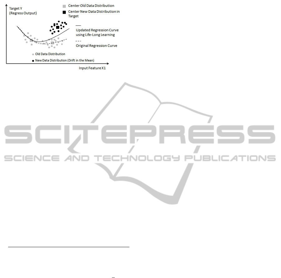
Figure 2: A typical drift in the target (right part of the
image) – life long learning (using RWLS relying on the
optimization problem in (6)) is too lazy and ends up in-
between the two data clouds (before = gray and after =
dark the drift), not being able to approximate the current
trend with sufficient accuracy.
with 1,…,,
the
error of the ith rule in sample and a
forgetting factor. The smaller is, the faster
the forgetting; usually a reasonable value lies in
[0.9, 1], where a value of 1 denotes no
forgetting. For instance, a forgetting of 0.9
would mean to include the last 21 samples with
a weight higher than 0.1 in the learning
process. Then, the deduction of the recursive
fuzzily weighted least squares estimator for
local region leads to (Lughofer, 2011d):
1
1
1
(8)
with
(9)
∙
1
1
1
∙1
⁄
and
1
1
(10)
where
1
,…,
,1 and
the value of variable at time instance
1.
Including forgetting in the antecedent part is
achieved by reactivating the winning cluster
with reducing the number of samples attached
to them, whenever
(
usually set to 30):
9.9∙
∙1 (11)
This automatically increases the learning gain
in (3) (
0.5/
, which was decreased
before with increasing
over time. In the
evaluation section, we will see that a forgetting
within the learning process is indispensable for
the application described in this paper, as no
forgetting will achieve an approximation error
which is 3-5 times higher.
Reducing unnecessary Complexity by Rule
merging: Reducing the complexity is important
in order to keep the models as slender as
possible, which also decreases the computation
time for model updates during the on-line
process. Furthermore, the models become more
transparent, when their complexity is low. In
fact, it is only possible to eliminate that
complexity which is not really necessary as
containing redundant, superfluous information.
The problem of unnecessary complexity during
the incremental update of fuzzy systems arises
whenever two (or more) clusters seem to model
distinct local regions at the beginning of the
data stream (due to a necessary non-linearity to
be modeled), however may move together due
to data samples filling up the gap in-between
these (also known as cluster fusion) (Lughofer,
2011c). The example in Fig. 3 shows such an
occurrence. Obviously, the fused regions can
be merged to one with hardly loosing any
accuracy.
In order to circumvent time-intensive overlap
criteria between two clusters and on high-
dimensional ellipsoids (Ros et al., 2002), we
use virtual projections of the two clusters in all
dimensions to one- dimensional Gaussians and
calculate an aggregated overlap degree based
on all intersection points according to the
highest membership degree in each dimension
(Lughofer, 2011c):
(12)
with
max
1
,
2
where denotes an aggregation operator
and
1
and
2
the
membership degrees of the two intersection
points of virtually projected Gaussians on
dimension . A feasible choice for is a t-
norm (Klement, 2000), as a strong non-overlap
along one single dimension is sufficient that
the clusters do not overlap at all – we used the
minimum operator in all test cases.
IJCCI2013-DoctoralConsortium
26

Figure 3: (Up) Two distinct clusters from original data and
(Down) samples are filling up the gap between the two
original clusters which get overlapping due to movements
of their centers and expansion of their ranges of influence.
If
is higher than a pre-defined
threshold (we used 0.8 as value in all tests),
then either a merge is conducted or the less
significant cluster deleted. This choice depends
on the similarity of the associated hyper-planes
defined in the local regions and : if the
similarity degree between the hyper-planes is
lower than those of the antecedents expressed
by (12), it points to an incon- sistency in the
rule base of the fuzzy system (Lughofer,
2011b). Thus, the less significant cluster is
deleted; otherwise the two clusters can be
merged. Similarity of the consequents can be
expressed by the angle spanned between the
normal vectors
,…,
,1
and
,…,
,1
of the two hyper-
planes: an angle close to 0 or 180 degrees
denotes a high similarity.
Merging of two rules and (defined by their
centers
,
, their spreads
,
, their
supports
,
, their consequent parameters
(hyper-planes)
,
, and their inverse
Hessian matrices
,
used for recursively
updating
in (10)) is conducted by (Lughofer,
2011c):
,
,
(13)
,
,
,
Δ
,
,
(14)
where 1,…,1, Δ
,
,
,
,
argmax
,
denoting the
(index of the) more significant cluster, and
consequently
argmin
,
denoting
the (index of the) less significant cluster. The
merging criterion and merging process is
integrated after each incremental update step,
i.e., after Step 9 in Algorithm 1.
7 EXPECTED OUTCOME
The objective of this PhD is to overcome the State-
of-Art methods in all the steps of the chemometric
modelling and then contribute in the rise of
Chemometrics as an important research field. Now it
is undervalued by the mathematics community and
also by part of the chemistry community, even when
it has proved its advantages in Analytical Chemistry
in the last decades.
Part of the points shown in Section 2 are already
finished and published. In preprocessing, and
concretely outlier detection, see (Cernuda, 2012a).
In dimensionality reduction we have tried several
novel approaches, see (Cernuda, 2012a; Cernuda,
2012b; Cernuda, 2013c). When it comes to off-line
batch modelling, use of problem specific
information and validation in presence of several
repeated measurements results can be seen in
(Cernuda, 2011; Cernuda, 2013a). In on-line
modelling we have succed on modelling highly
dynamic processes, see (Cernuda, 2012a). Last but
not least, cost reduction results has been recently
presented in the 13th Scandinavian Symposium on
Chemometrics, see [SSC13].
REFERENCES
Abraham, W., Robins, A., 2005. Memory retention—the
synaptic stability vs plasticity dilemma, Trends in
Neurosciences 28 (2) 73–78.
Backer, S. D., Scheunders, P., 2001. Texture segmentation
by frequency-sensitive elliptical competitive learning,
Image and Vision Computing 19 (9–10) 639–648.
Cernuda, C., Lughofer, E., Maerzinger, M., Kasberger, J.,
2011. Nir-based quantification of process parameters
in polyetheracrylat (pea) production using flexible
AdvancedLearningTechniquesforChemometricModelling
27

non-linear fuzzy systems, Chemometrics and
Intelligent Laboratory Systems 109 (1) 22–33.
Cernuda, C., Lughofer, E., Suppan, L., Roeder, T.,
Schmuck, R., Hintenaus, P., Maerzinger, W.,
Kasberger, J., 2012. Evolving chemometric models for
predicting dynamic process parameters in viscose
production, Analytica Chimica Acta, 725, 22–38.
Cernuda, C., Lughofer, E., Maerzinger, M., Summerer,
W., 2012. Waveband selection in NIR spectra using
enhanced genetic operators, Chemometrics for
Analytical Chemistry 2012, Budapest, CIO-4.
Cernuda, C., Lughofer, E., Hintenaus, P., Maerzinger, W.,
Reischer, T., Pawliczek, M., Kasberger, J., 2013.
Hybrid adaptive calibration methods and ensemble
strategy for prediction of cloud point in melamine
resin production, Chemometrics and Intelligent
Laboratory Systems, volume 126, pp. 60 – 75.
Cernuda, C., Lughofer, E., Mayr, G., Roeder, T.,
Hintenaus, P., Maerzinger, W., 2013. Decremental
active learning for optimized self-adaptive calibration
in viscose production, 13
th
Scandinavian Symposium
in Chemometrics, Stockholm.
Cernuda, C., Lughofer, E., Hintenaus, P., Maerzinger, W.,
2013. Enhanced Genetic Operators Design for
Waveband Selection in Multivariate Calibration by
NIR Spectroscopy, Journal of Chemometrics,
(submitted).
Cleveland, W., Devlin, S., 1988. Locally weighted
regression: an approach to regression analysis by local
fitting, Journal of the American Statistical Association
84 (403) 596–610.
Draper, N., Smith, H., 1998. Applied regression analysis,
Wiley Interscience, Hoboken, NJ.
Gray, R., 1984. Vector quantization, IEEE ASSP
Magazine 1 (2) (1984) 4–29.
Haenlein, M., Kaplan, A., 2004. A beginner’s guide to
partial least squares (PLS) analysis, Understanding
Statistics 3 (4) (2004) 283–297.
Hamker, F., 2001. RBF learning in a non-stationary
environment: the stability-plasticity dilemma, in: R.
Howlett, L. Jain (Eds.), Radial Basis Function
Networks 1: Recent Developments in Theory and
Applications, Physica Verlag, Heidel- berg, New
York, pp. 219–251.
Hastie, T., Tibshirani, R., Friedman, J., 2007. Pathwise
coordinate optimization, The Annals of Applied
Statistics 1 (2) 302–332.
Hastie, T., Tibshirani, R., Friedman, J., 2010. Regularized
paths for generalized lin- ear models via coordinate
descent, Journal of Statistical Software 33 (1).
Haykin, S., 1999. Neural Networks: A Comprehensive
Foundation, Prentice Hall.
Jolliffe, I., 2002. Principal Component Analysis, Springer
Verlag, Berlin Heidelberg New York.
Klement, E., Mesiar, R., Pap, E., 2000. Triangular Norms,
Kluwer Academic Publishers, Dordrecht, Norwell,
New York, London.
Ljung, L., 1999. System Identification: Theory for the
User, Prentice Hall PTR, Prentice Hall Inc, Upper
Saddle River, NJ.
Lughofer, E., 2008. FLEXFIS: a robust incremental
learning approach for evolving TS fuzzy models, IEEE
Transactions on Fuzzy Systems 16 (6) 1393–1410.
Lughofer, E., Kindermann, S., 2008. Improving the
robustness of data-driven fuzzy systems with
regularization, in: Proceedings of the IEEE World
Congress on Computational Intelligence (WCCI)
2008, Hongkong, pp. 703–709.
Lughofer, E., 2011. On-line incremental feature weighting
in evolving fuzzy classifiers, Fuzzy Sets and Systems
163 (1) 1–23.
Lughofer, E., Hüllermeier, E., 2011. On-line redundancy
elimination in evolving fuzzy regression models using
a fuzzy inclusion measure, in: Proceedings of the
EUSFLAT 2011 Conference, Elsevier, Aix-Les-Bains,
France, pp. 380–387.
Lughofer, E., Bouchot, J.-L., Shaker, A. 2011, On-line
elimination of local redundancies in evolving fuzzy
systems, Evolving Systems, vol. 2 (3), pp. 165-187.
Lughofer, E., Angelov, P., 2011. Handling drifts and shifts
in on-line data streams with evolving fuzzy systems,
Applied Soft Computing, vol. 11, pp. 2057-2068.
Miller, J., Miller, J., 2009. Statistics and Chemometrics for
Analytical Chemistry, Prentice Hall, Essex, England.
Qin, S., Li, W., Yue, H., 2000. Recursive PCA for
adaptive process monitoring, Journal of Process
Control 10 (5) 471–486.
Reeves, J., Delwiche, S., 2003. Partial least squares
regression for analysis of spectroscopic data, Journal
of Near Infrared Spectroscopy 11 (6) 415–431.
Ros, L., Sabater, A., Thomas, F., 2002. An ellipsoidal
calculus based on propagation and fusion, IEEE
Transactions on Systems, Man and Cybernetics—Part
B: Cybernetics 32 (4) 430–442.
Shao, X., Bian, X., Cai, W., 2010. An improved boosting
partial leastsquares method for near-infrared
spectroscopic quantitative analysis, Analytica Chimica
Acta 666 (1–2) 32–37.
Takagi, T., Sugeno, M., 1985. Fuzzy identification of
systems and its applications to modeling and control,
IEEE Transactions on Systems, Man and Cybernetics
15 (1) 116–132.
Vaira, S., Mantovani, V.E., Robles, J., Sanchis, J.C.,
Goicoechea, H., 1999. Use of chemometrics: principal
component analysis (PCA) and principal component
regression (PCR) for the authentication of orange
juice, Analytical Letters 32 (15) 3131–3141.
Widmer, G., Kubat, M., 1996. Learning in the presence of
concept drift and hidden contexts, Machine Learning
23 (1) 69–101.
IJCCI2013-DoctoralConsortium
28
