
Multiplicative Neural Network with Thresholds
Leonid Litinskii and Magomed Malsagov
Center for Optical Neural Technologies,
Scientific Research Institute for System Analysis of Russian Academy of Sciences,
Vavilov Str, Moscow, Russia
Keywords: Hopfield-type Network, Multiplicative Connections, Ground State.
Abstract: The memory of Hopfield-type neural nets is understood as the ground state of the net – a set of
configurations providing a global energy minimum. The use of thresholds allows good control over the
ground state. It is possible to build multiplicative networks with the degeneracy of the ground state
exceeding considerably the dimensionality of the problem (that is, the net memory can be much greater than
the dimensionality of the problem). The paper considers the potentials and limitations of the approach.
1 INTRODUCTION
Let us consider a Hopfield-type neural network with
a multiplicative connection matrix
(1 )
ij ij i j
M
uu
, , 1,..,ij p . Here
ij
is the
Kronecker symbol,
p
is the space dimensionality,
real numbers
i
u are the coordinates of normalized
vector
1
( ,..., )
p
uuu= :
2
p
u
. The fixed point of
the net is a configuration whose binary coordinates
are the signs of coordinates of vector
u
:
12
( , ,..., ) is a fixed point;
sgn( ), 1,.., .
p
ii
ss s
suip
s
The set of fixed points changes significantly if we
define the dynamics of the same matrix by using
thresholds
i
T , which are not only non-zero, but also
proportional to coordinates
i
u :
1
() , () ,
(1)sgn ()
ij ij i i
p
iijji
j
JfxMTgxu
s
Js T
(1)
Being functions of parameter
x
, multipliers ()
f
x
and
()
g
x themselves serve as free parameters of the
model.
()
i
s
is the
i
-th coordinate of configuration
()
s determining the state of the net at time
. The
arrangement of the set of fixed points of this sort of
net is more complicated and more interesting. It
turns out to be possible to determine fully the
configuration sets that bring the energy functional to
a global minimum. Such configurations are usually
called the ground state of the net (the term is
borrowed from physics). It is the ground state that is
regarded as the memory of a net: it is also the case
with the Hebb matrix and projection connection
matrix (Hertz et al., 1991).
Given model (1), it is possible to determine
analytically the dependence of the ground state on
external parameters
f
,
g
,
x
and
u
. It is possible
to control the ground state by varying external
parameters. In short, the findings are as follows.
Generally speaking, the whole set of
2
p
configurations
s
falls into sets of configurations
that are equally distant from vector
u
. Let us call
such sets
equidistant classes. It proves that only
equidistant classes can serve as the ground state of
the net: under particular conditions all
configurations of one class (and no other) provide a
global minimum to the energy functional. The
composition and the number of equidistant classes
are defined by vector
u
. The conditions that make
one or another class become the ground state are
determined by
()fx and ()
g
x .
The possibility to make the ground state multiply
degenerate by choosing vector
u
is a valuable
advantage of the approach. The ground state can
hold a great deal of configurations: the number of
configurations is a polynomial function of the
dimensionality
p
. That is to say, it becomes
possible to build networks of very large memory.
523
Litinskii L. and Malsagov M..
Multiplicative Neural Network with Thresholds.
DOI: 10.5220/0004629605230528
In Proceedings of the 5th International Joint Conference on Computational Intelligence (NCTA-2013), pages 523-528
ISBN: 978-989-8565-77-8
Copyright
c
2013 SCITEPRESS (Science and Technology Publications, Lda.)

The disadvantage of the method is that not any set of
configuration can serve as the ground state. This
state can’t consist of fully random configurations
because the configurations must be equally distant
from vector
u
. Equidistant configurations are
located around vector
u
symmetrically. And that is
the limitation of the whole approach. How we can
overcome this restriction is considered at the end of
the paper.
In the next section we give the main results of
the work and their short explanations, and consider
one specific example. In the final section we analyze
the potentials and limitations of the approach.
2 MAIN RESULTS
The energy of state
s
of network (1) is equal to
,1 1
2
()~ 2
()( ) 2 ()( ),
pp
ij i j i i
ij i
EJssTs
fx gx
s
u,s u,s
where
()u,s is the scalar product of
p
-dimensional
normalized vectors
u
and
s
:
1
()
p
ii
i
us
u,s
. In
further consideration it will be better to seek maxima
of
() ()
F
Ess:
2
() ( )( ) 2 ( )( ) maxFfx gxsu,s u,s
(2)
2.1 Classes
k
Σ
Functional ()
F
s takes the same value for all
configurations the scalar products of which by
vector
u
have the same value. Let us introduce the
cosine of the angle between vectors
s
and
u
:
cos , / .wp su
When
s
runs over 2
p
possible configurations,
cos w
doesn’t necessarily takes 2
p
different values.
Let us number different values of the cosine in
descending order starting the numbering with 0:
01 1
cos cos ... 0 ... cos cos .
tt
ww w w
(3)
The number
1t
of different values of the cosine
does not exceed
2
p
. Let
k
stand for the class of
configurations
s
such that the cosine of the angle
between
s
and vector
u
is cos
k
w :
: , cos , 0,1,..., .
kk
p
wk t ssu
(4)
Clear that each configuration from class
k
is the
same distance away from vector
u
, other
configurations being a different distance off
u
.
We see that functional
()
F
s (2) takes
1t
values no matter what value
x
takes. All we have to
do to find the ground state is to find the greatest
among
1t
values:
2
()
~ ( ) cos 2 cos , 0,1,.., .
kk k
gx
Ffx w wk t
p
(5)
The number of classes
k
and their composition are
determined by vector
u
solely. With that,
k
F
are
determined by cosines
cos ~ ,
k
w su
for fixed
f
,
g
and
x
. We restrict our consideration to the case
when vectors
u
have only nonnegative coordinates.
The results can be easily extended to the case when
some of
i
u are negative (see below). We will assume
that
i
u are arranged in ascending order:
12
0....
p
uu u
It is easy to see that the sequence of cosines (3) is
symmetric about its middle point:
cos cos , , .
ktkktk
ww kt
If the number of different classes is even
(
12tl
), the cosines first go down to their
positive minimum
1
cos
l
w
, then they become
negative:
01 1
10
cos cos ... cos 0
cos cos ... cos cos .
l
ll t
ww w
ww ww
None of the cosines of the sequence is zero. On the
other hand, when
2tl
, one of the cosines (3) is
zero, and the sequence has the form:
01
11 0
cos ... cos cos 0
cos cos ... cos cos .
ll
ll t
www
ww ww
In this case
l
-class configurations are orthogonal
to vector
u
.
By way of example let us build a few starting
classes
k
when the coordinates of vector
u
obey
the following rule:
1234
0...
p
uu uu u
with
24
2uu
. Class
0
holds configurations that
are nearest to vector
u
, so
0
e
, where
(1,1,..,1)
e . The corresponding cosine is equal to
0
1
cos /
p
i
wup
. Class
1
consists of
IJCCI2013-InternationalJointConferenceonComputationalIntelligence
524

configurations that are a bit more distant from
u
than
0
-class configurations. In our case it gives
1
( 1,1,...,1)
, and
101
cos cos 2 /wwup .
The next class holds two configurations
(1, 1, 1, ..,1)
and
(1,1, 1, ..,1) , and
202
cos cos 2 /wwup.
Class
3
also consists of two configurations
(1,1,1,..,1) and (1,1, 1,..,1) , and
3012
cos cos 2( ) /wwuup. Class
4
holds one
configuration
4
(1, 1, 1,1,...,1)
, and
402
cos cos 4 /wwup. So does class
5
:
5
(1,1,1, 1,...,1)
,
504
cos cos 2 /wwup . And
so on. To distribute all configurations into classes
k
, it is necessary to arrange in ascending order all
2
p
possible sums
1
p
ii
i
u
where coefficient
i
can
be either 0 or 1. This task is similar to the number
partitioning problem (Mertens, 2001). In our case it
is not necessary to try to solve the problem in
general.
Another example. It is not difficult to describe
the distribution of configurations among equidistant
classes when vector
(1,1,...,1)ue . It is easy to
see that in this case the cosines take
1p different
values:
cos 1 2 , 0,1,..., ,
k
wkpk p
(6)
and the
k
-th class holds the configurations that have
exactly
k
negative coordinates. Let us introduce a
special notification for such classes:
()
1
: , 2 , 0,1,..., .
p
ki
i
s
pkk p
e
sse
(7)
The number of configurations in class
()
k
e
is
p
k
.
Further one or another
σ
-configuration will be
often used as vector
u
. Basing on classes
()
k
e
it is
simple to understand the structure of equidistant
classes in this case. Clear that both the number of
different cosines and their values remains the same
as with
ue
(see (6)). Coordinatewise
multiplication of all configurations from class
()
k
e
by
σ
-configuration is used to obtain class
()
k
σ
from
class
()
k
e
(7):
()
1
: , 2 , 0,1,..., .
p
kii
i
s
pkk p
σ
ssσ
2.2 Functions f(x) and
g
(x)
Now let us consider the role of functions ()
f
x
and
()
g
x . Collection of
0
()
t
k
Fx
(5) is a family of
functions of
x
. Function ()
l
F
x , which surpasses
other functions at particular
x
, determines ground-
state class
l
.
Let the amplitude of function
()
l
F
x at point
0
x
be greater than amplitudes of other functions:
00
() ()
lk
F
xFx kl. If ()
f
x and ()
g
x are
continuous functions, a small variation of
x
does
not change the superiority of
()
l
F
x over other
functions in the general case. Class
l
keeps being
the ground state in a small vicinity of
0
x
. If
x
changes on, it becomes almost inevitable that
function
()
l
F
x intersects another function, say,
()
n
F
x . After that it is ()
n
F
x that starts exceeding
all other functions. At the point of intersection of
functions the ground state passes to class
n
: the
transition of the ground state
ln
takes place.
Of course, the transition point is defined by forms of
functions
()
f
x , ()
g
x and cosines (3). However,
something about the way the ground state changes
can be understood from the general considerations.
Let us rearrange formula (5) by taking
()
f
x out
of the brackets and completing the expression in the
brackets to the square. Accurate to insignificant
items, the formula we get is
2
~()cos (),
()
() , 0,1,..,.
()
kk
Ffx w x
gx
x
kt
pfx
(8)
Let us first assume that
() 0fx . In this event it is
necessary to maximize the modulus of the bracketed
expression with respect to
k to find the largest
k
F
:
max cos ( ) .
k
k
wx
(9)
If
()
x
is negative, the maximum of modulus (9) is
ensured by the greatest value of the cosine, and the
solution of (9) is
0k
. In this case, the ground state
is associated to class
0
. Conversely, if ()
x
is
positive, the maximum of modulus (9) is ensured by
the smallest value of the cosine. The solution of (9)
is
kt
in this event, and the ground state is
attributed to class
0t
. So, when ()
f
x is
positive, either class
0
(if () 0gx ) or class
t
(if
MultiplicativeNeuralNetworkwithThresholds
525
() 0gx
) becomes the ground state.
Let us now examine what happens if
() 0fx
.
In this case it is necessary to minimize the modulus
of the bracketed expression (8) with respect to
k to
find the largest
k
F
. Generally speaking, to do it is
not at all difficult: it is just necessary to define
cos
k
w that is closest to the current value of ()
x
.
The corresponding class
k
will be the ground state
of the net. Let us look at Figure 1 to understand
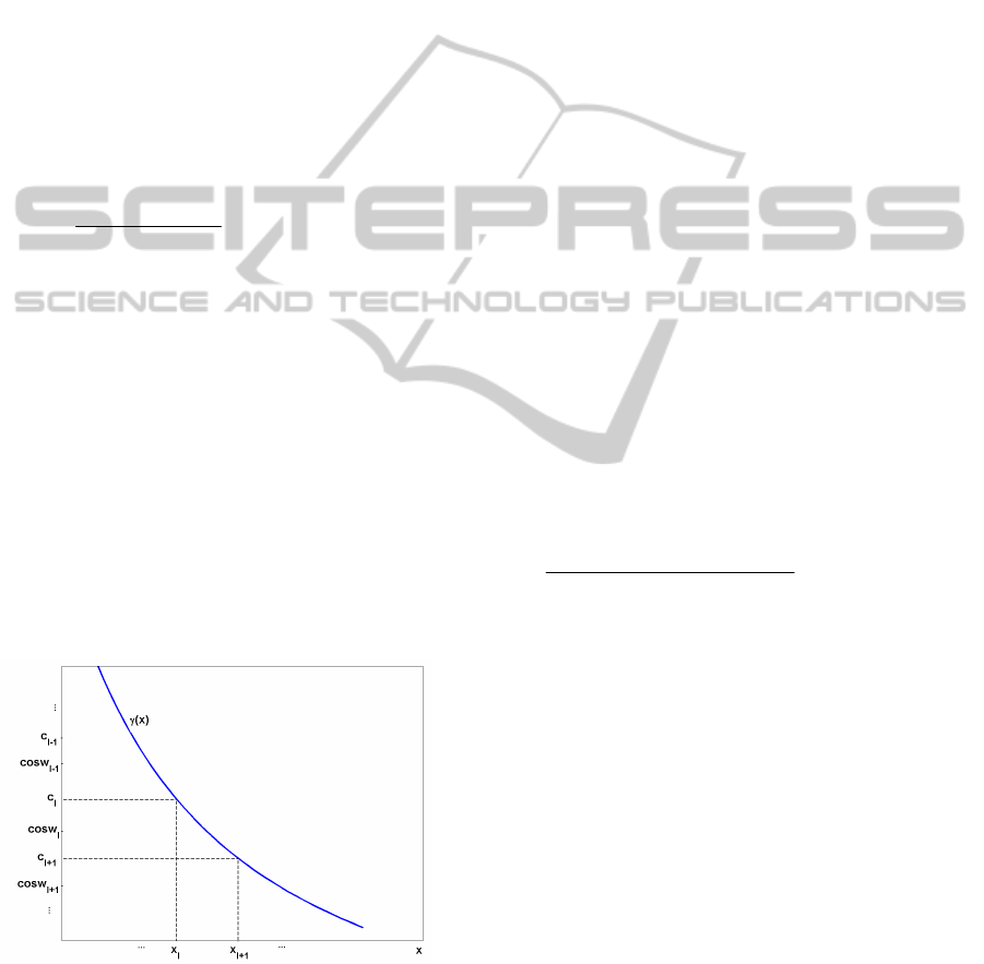
collisions that occur in this case.
In Figure 1 the
Y
-axis carries representative
values of
cos
k
w for 1, and 1kl l l . The
steadily decreasing curve represents function
()
x
.
k
c denotes the half sum of two successive values of
the cosine:
1
cos cos
,1,2,...,.
2
kk
k
ww
ckt
(10)
The value of
x
at which ()
k
x
c
is indicated
as
k
x
:
1
() ().
kk k k
x
cx c
(11)
Let
x
belong to interval
1
,
ll
x
x
initially:
1ll
x
xx
. It is easy to see that for any
x
from
this interval it is
cos
l
w that is nearest to ()
x
. So,
kl
is the solution of (9), and class
l
serves as
the ground state of the net. Note that it is true for all
x
in the interval
1
,
ll
x
x
. Variable
x
can grow
(fall) until it steps over
1l
x
(
1l
x
) and the ground
state passes to class
1l
(
1l
), and so on.
Figure 1: Graphical solution of the problem (9): see body
of the paper.
We see that when
() 0fx
and
()
x
is a
continuous function, the changing of the ground
state changes its number by 1:
1kk
. There is a
kind of continuity in its number changing with
parameter
x
. In principle, it is possible to organize
“discontinuous” control over ground-state “jumps”
kl
so that class numbers
k
and
l
would
differ by more than 1. For this purpose one should
use either discontinuous function
()
g
x , or the fact
that when
()
f
x
becomes positive, the ground state
passes from any class
k
to either class
0
or
t
.
2.3 Example
To exemplify the results let us consider functions
()fx and ()
g
x of the following form (Litinskii,
1999):
() 1 2, () (1 ), 1.fx xgx q x q
In this case
()
k
F
x in (5) takes the form:
2
( ) cos 2 cos cos .
kkkk
F
x qpw xqpwqpw
Competing functions
()
k
F
x are a family of straight
lines whose structure can be examined easily. As a
result, we get the following statement.
Theorem. When
x
grows indefinitely from the
initial value of 0, the ground state of a net passes
consecutively to classes
k
(4):
max
012
...
k
. Transition
1kk
occurs at critical point
1
max
1
/cos cos/2
,1,2,...,,
/cos cos
kk
k
kk
qp w w
xkk
qp w w
and as long as
1
,
kk
xxx
, class
k
is the ground
state of the net. Number
max
k of the last transition is
determined by the requirement that denominator
1
/cos cos
kk
qp w w
should be positive. If vector
u
is configuration, the ground-state configurations
are the only fixed points of the net.
The composition of classes
k
is not detailed in
the theorem at all: classes consist of configurations
equally distant from vector
u
. After classes
k
are
defined with the aid of
u
, change of parameter
x
results in the ground state jumping from one class to
another. It is possible to show that independently of
vector
u
the first transition of the ground state
01
occurs after ½:
1
1/2x . Additionally, it
turns out that
max
k is always greater than
/2p
, and
max
1
k
x . The use of factor
q
makes it possible to
regulate the total number of ground-state transitions.
IJCCI2013-InternationalJointConferenceonComputationalIntelligence
526

3 DISCUSSION
AND CONCLUSIONS
The findings from the previous paragraph allow us
to control the ground state of the net to a
considerable extent. Let us consider a
p
-
dimensional hyper-cube with edge length of 2 and
center at the origin of coordinates. Configurations
s
are located at cube vertexes. Symmetric directions in
the hyper-cube must be chosen as vector
u
. For
each
u
of that kind 2
p
s
-configurations are
distributed in symmetric sets with vector
u
being
the axis of symmetry. Each set like that forms one of
k
classes. It can be turned into the ground state by
using the approach offered. Particularly, it is
possible to create the ground state from a very large
number of configurations. For example, the number
of
()
k
e
-class configurations (7) is equal to
!! !pkpk
.
Some coordinates of vector
u
can be zero. Let
1
0u . Then the same class will comprise not only
configuration
12
(, ,..., )
p
s
sss , but also
configuration
12
' ( , ,..., )
p
s
sss . In other words,
vector
u
having a zero coordinate results in the
number of configurations doubling in each class
k
.
In this event the conclusive statement of Theorem is
more general and should read: if non-zero
coordinates of vector
u
are equal to each other, the
ground-state configurations are the only fixed points
of the net.
What possible consequences the approach can
have are not known yet. It is necessary to look
through all symmetric directions of
u
in the hyper-
cube and arrange cube vertexes with respect to
vertex-to-vector
u
distance in each case. It is
necessary to turn to methods of the group theory
here (Davis, 2007).
The disadvantage of the whole approach is that
configurations comprising the ground state can’t be
arbitrary. They are the same distance from vector
u
and, therefore, form a symmetric set. We hope that
the following tricks (or their combinations) can help
us to avoid total symmetry of the ground state. First,
we can use a few vectors like
u
into the connection
matrix and thresholds rather just one vector. For
example, let there be vector
12
(, ,..., )
p
vv vv ,
2
pv
, and let us consider a neural net similar to
(1):
1
()(1 )( ),
()( ),
(1)sgn () .
ij ij i j i j
iii
p
iijji
j
Jfx uuvv
Tgxuv
s
Js T
(12)
If vectors
u
and
v
are configurations, it proves that
as long as
x
does not exceed the first transition
point
1
x
, the initial configurations
u
and
v
themselves are the ground state. If
1
x
x , a set
of configurations equally distant from both
u
and
v
will constitute the ground state. The net (12) will not
have other fixed points. Supported by a computer
simulation, this result arouses cautious optimism.
Second, it is possible to “separate” in (1)
thresholds
i
T and numbers
i
u used for building the
multiplicative matrix
ij
M
. Let us use earlier-
introduced vector
v
and consider a neural net
1
()(1 ) , () ,
(1)sgn () .
ij ij i j i i
p
iijji
j
J
fx uu T gxv
sJsT
Tentative considerations show that its ground state is
formed by
k
-class configurations nearest to the
vector difference
uv
. In other words, the trick
allows us to avoid the total symmetry of the ground
state. Of course the results need closer research.
The memory of the standard Hopfield model
with the Hebbian connection matrix and random and
independent patterns
()
s is well understood.
However, if the connection matrix is of the general
form, the memory of such a network is practically
unknown. In the same time an arbitrary connection
matrix
J
can be presented as a quasi-Hebbian one,
when using: i) orthogonal vectors
(μ)
u related to the
eigenvectors of the matrix
J
,
() ()
11
(1 )
ij ij i j
Juu
()+ ()
J~ u u
where
() ()
1
,...,
p
uu
(μ)
u=( )
,
()
i
u
1
R , ,
(μ)(ν)
uu
ii) or configuration vectors
(μ)
s with the weights r
(Kryzhanovsky, 2007):
1
r
()+()
J~ s s
,
()
1
i
s
,
1
r
R
.
Our multiplicative matrix
M
is only one term of the
quasi-Hebbian expansion. We hope that a detailed
analysis of the network with the connection matrix
M
will allow us to make headway on investigating
a more general case.
MultiplicativeNeuralNetworkwithThresholds
527

ACKNOWLEDGEMENTS
The work was supported by Russian Basic Research
Foundation (grants 12-07-00259 and 13-01-00504).
REFERENCES
Hertz, J., Krogh, A., Palmer, R., 1991. Introduction to the
Theory of Neural Computation. Massachusetts:
Addison-Wesley.
Mertens, S., 2001. A Physicist's Approach to Number
Partitioning. Theoret. Comput. Sci. 265, 79-108.
Litinskii, L. B., 1999. High-symmetry Hopfield-type
neural networks. Theoretical and Mathematical
Physics, 118: 107-127.
Davis, M. W., 2007. The geometry and topology of
Coxeter groups. Princeton: Princeton University Press.
Kryzhanovsky, B. V., 2007. Expansion of a matrix in terms
of external products of configuration vectors. Optical
Memory & Neural Networks (Information Optics), 16:
187-199.
IJCCI2013-InternationalJointConferenceonComputationalIntelligence
528
