
Statistical and Scaling Analyses of Neural Network Soil Property
Inputs/Outputs at an Arizona Field Site
Alberto Guadagnini
1,2
, Shlomo P. Neuman
2
, Marcel G. Schaap
3
and Monica Riva
1,2
1
Dipartimento di Ingegneria Civile e Ambientale, Politecnico di Milano, 20133 Milano, Piazza L. Da Vinci 32, Italy
2
Department of Hydrology and Water Resources, University of Arizona, Tucson, Arizona 85721, U.S.A.
3
Department of Soil, Water and Environmental Science, University of Arizona, Tucson, Arizona 85721, U.S.A.
Keywords: Neural Network, Soil Texture, Soil Hydraulic Properties, Spatial Statistics, Scaling.
Abstract: Analyses of flow and transport in the shallow subsurface require information about spatial and statistical
distributions of soil hydraulic properties (water content and permeability, their dependence on capillary
pressure) as functions of scale and direction. Measuring these properties is relatively difficult, time
consuming and costly. It is generally much easier, faster and less expensive to collect and describe the
makeup of soil samples in terms of textural composition (e.g. per cent sand, silt, clay and organic matter),
bulk density and other such pedological attributes. Over the last two decades soil scientists have developed a
set of tools, known collectively as pedotransfer functions (PTFs), to help translate information about the
spatial distribution of pedological indicators into corresponding information about soil hydraulic properties.
One of the most successful PTFs is the nonlinear Rosetta neural network model developed by one of us.
Among remaining open questions are the extents to which spatial and statistical distributions of Rosetta
hydraulic property outputs, and their scaling behavior, reflect those of Rosetta pedological inputs. We
address the last question by applying Rosetta, coupled with a novel statistical scaling analysis recently
proposed by three of us, to soil sample data from an experimental site in southern Arizona, USA.
1 INTRODUCTION
Soil hydraulic properties (such as volumetric water
content, permeability and their functional relations
to capillary pressure) required for subsurface flow
and transport analyses can be measured in the field
and/or the laboratory at a considerable investment of
time and money. One alternative is to estimate these
properties indirectly by means of pedotransfer
functions (PTFs, for a review see Pachepsky and
Rawls, 2004) on the basis of pedological indicators
such as soil particle size distribution, bulk density
and organic matter content that are much simpler
and less costly to determine. PTFs range from
simple look-up tables to advanced statistical
analyses such as support vector machines (e.g.
Twarakavi et al., 2009). One of the most powerful
and increasingly popular tools of this kind is the
nonlinear Rosetta neural network code of Schaap et
al. (2001), which comprises a set of five hierarchical
PTFs tailored to varied circumstances ranging from
data-poor to data-rich. Inputs may be limited to soil
composition data such as per cent sand, silt and clay
or include additional information about soil bulk
density and one or two measured pairs of water
content and capillary pressure data. Output consists
of parameters defining the van Genuchten (1980) –
Mualem (1976) constitutive relationships between
water content, hydraulic conductivity and capillary
pressure. The code has been calibrated against
pedological and hydraulic data obtained from
laboratory analyses of 2134 soil samples from across
the United States. The calibration was combined
with the non-parametric bootstrap method (Efron
and Tibshirani, 1993) to allow assessing Rosetta's
predictive uncertainty. Assuming that the calibration
data set of 2134 samples represents correctly the
underlying soil population, multiple random subsets
(or replicas) of the original dataset were created
through sampling with replacement: 100 replicates
of saturated hydraulic conductivity and 50 replicates
of van Genuchten – Mualem constitutive parameters
(Schaap and Leij, 1998). Rosetta was calibrated
separately against each replicate data set, each
calibrated version was used to predict hydraulic
parameters on the basis of the original 2134 input
data, and the results summarized in terms of sample
mean and standard deviation of each predicted
489
Guadagnini A., P. Neuman S., G. Schaap M. and Riva M..
Statistical and Scaling Analyses of Neural Network Soil Property Inputs/Outputs at an Arizona Field Site.
DOI: 10.5220/0004600804890494
In Proceedings of the 3rd International Conference on Simulation and Modeling Methodologies, Technologies and Applications (MSCCEC-2013), pages
489-494
ISBN: 978-989-8565-69-3
Copyright
c
2013 SCITEPRESS (Science and Technology Publications, Lda.)
parameter (Schaap et al., 2001). The latter two
statistics are taken to represent the mean and the
uncertainty of the corresponding neural network
predictions, which vary with each individual set of
input data.
Due to their reliance on diverse data bases
obtained using varied measurement techniques, it is
not uncommon for different PTFs to produce
mutually inconsistent outcomes (Schaap and Leij,
1998). Most PTFs have a modest accuracy when
estimated hydraulic parameters are compared with
experimental values (Schaap et al., 2004). In the
case of Rosetta, correlation coefficients between
experimental and estimated constitutive parameters
of the van Genuchten water retention model range
between 0.3 and 0.9 (Schaap et al., 2001). The root-
mean square error between measured and estimated
water contents range from 0.04 to 0.08 cm3/cm3,
depending on model used. Correcting for capillary
pressure-dependent bias reduces this error only
slightly (Schaap et al., 2004).
It is presently unclear to what extent do spatial
and statistical distributions of Rosetta hydraulic
property outputs, and their scaling behavior, reflect
those of Rosetta pedological inputs. In this paper we
address, in a preliminary manner, the question to
what degree are the statistical scaling properties of
Rosetta inputs reflected in those of the model's
outputs. We do so by analyzing, and comparing, the
statistical scaling properties of Rosetta inputs and
outputs using input soil sample data from an
experimental site near Maricopa, Arizona, USA
(Schaap, 2013). Our statistical scaling analysis is
based on an approach recently proposed by Neuman
et al. (2013 and references therein).
2 STATISTICAL SCALING OF
NEURAL NETWORK INPUTS
We start by analyzing the statistical scaling behavior
of soil texture data measured to a depth of 15 meters
over an area of 3600 m
2
at the Maricopa
experimental site, operated by the University of
Arizona (headquartered in Tucson). These data
constitute inputs into the Rosetta neural network
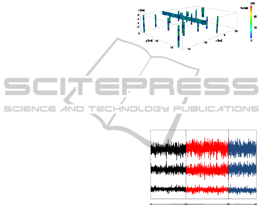
model. The sampling network, depicted in Figure 1,
comprises 1029 measurement locations distributed
along several vertical wells and a horizontal transect.
A more complete description of the site and the
network is given by Schaap (2013).
Our texture data consist of relative fractions f
i
, 0
f
i
1, of three texture categories i = sa, si and cl
representing sand, silt and clay, respectively. In
addition to the original measurements, f
i
, we also
consider two corresponding principal components,
PC1 and PC2, as defined by Schaap (2013). Here we
focus on statistical scaling of vertical increments in
these variables.
Figure 1: Spatial distribution of soil sampling network at
Maricopa experimental site. Grey scale represents
measured relative silt fraction, f
si
.
Figure 2 juxtaposes sequences of vertical increments
in f
sa
, f
si
and f
cl
, computed along the various
sampling boreholes in Figure 1, at vertical
separation distances (lags) s
v
= 0.4, 2.0 and 5.0 m.
The increments are seen to vary randomly and
intermittently.
Figure 2: Sequences of N vertical increments in f
sa
, f
si
and
f
cl
at lags s
v
= 0.4, 2.0 and 5.0 m.
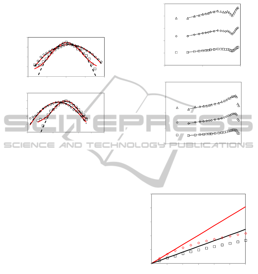
Frequency distributions of vertical increments, like
those of the principal components PC1 and PC2 in
Figure 3, tend to be symmetric and exhibit heavy
tails. As illustrated in Figure 3, they can be fitted
quite well by the maximum likelihood (ML) method
to
-stable probability density functions (pdfs) with
stability indices
≤ 2, where
= 2 corresponds to
the normal (Gaussian) pdf. ML fits of normal pdfs to
the empirical distributions are included in Figure 3
for reference. Whereas the tails of
-stable pdfs with
< 2 fall off as a power law, those of the normal pdf
decay exponentially. ML estimates of
associated
with vertical increments of PC1 and PC2 increase
from 1.85 at a lag of 0.4 m to 2 at lags exceeding 2
0.0
0.0
0.0
+0.5
0.5
+0.5
0.5
+0.5
0.5
s
v
= 0.4 m
N = 1246
s
v
= 2.0 m
N = 1489
s
v
= 5.0 m
N = 983
Vertical incremental values of f
i
(i = sa, si, cl)
f
sa
(sand)
f
si
(silt)
f
cl
(clay)
SIMULTECH2013-3rdInternationalConferenceonSimulationandModelingMethodologies,Technologiesand
Applications
490
m. Kolmogorov – Smirnov and Shapiro – Wilk tests
at significance level of 0.05 do not, in most cases,
support a hypothesis that increments associated with
estimates of
> 1.9 derive from a normal pdf.
Figure 3: Frequency distributions of increments of (a) PC1
and (b) PC2 at two lags. Also shown are ML fits of
-
stable (red solid) and normal (dashed) pdfs.
Next we compute structure functions
q
N
S defined as
q
th
order sample statistical moments of absolute
vertical increments in a sample of size N. Figure 4
plots sample structure functions of orders 1, 2 and 3
associated with vertical increments of PC1 and PC2
as functions of vertical lag on logarithmic scale. In
each case there is a mid-range of lags within which
the data can be fitted by regression to straight lines
at high levels of confidence as indicated by
coefficients of determination, R
2
, close to 1. This
implies that, in a midrange of lags, each structure
function scales as a power of lag; Figure 4 lists
corresponding power exponents, which we designate
by
(q), ranging from 0.34 to 0.74 in the case of PC1
and from 0.21 to 0.49 in the case of PC2. We refer to
this way of determining power scaling exponents for
various orders q of a structure function as method of
moments (M).
Figure 5 shows how the power-law scaling
exponent,
(q), determined for PC1 and PC2 by the
method of moments, varies with the order q of their
structure functions up to q = 6. The exponent
(q) is
seen to scale in a nonlinear fashion with q,
delineating a convex curve. Included in Figure 5 are
straight lines passing through
(1) and the origin.
Figure 4: Structure functions of order q = 1, 2 and 3 of
vertical (a) PC1 and (b) PC2 increments versus lag.
Regression lines (R
2
values listed) indicate power-law
scaling (equations listed) in midranges of lags.
Figure 5: Variations of power-law scaling exponent
(q)
corresponding to PC1 and PC2 with order q of their
respective structure functions obtained by the method of
moments. Straight lines pass through
(1) and the origin.
Power-law scaling of
-stable increments such
that illustrated in Figures 4 and 5, including
breakdown in power-law scaling at small and large
lags and nonlinear variation of the power-law
scaling exponent
(q) with q, have been shown by us
elsewhere to be typical of samples from sub-
Gaussian random fields or processes subordinated to
1.0E-05
1.0E-04
1.0E-03
1.0E-02
1.0E-01
-80.0 -40.0 0.0 40.0 80.0
1.0E-05
1.0E-04
1.0E-03
1.0E-02
1.0E-01
1.0E+00
-30.0 -20.0 -10.0 0.0 10.0 20.0 30.0
pdf
pdf
Increments of PC1
Increments of PC2
(a)
(b)
s
v
= 0.40 m
s
v
= 5.00 m
1.0E+00
1.0E+01
1.0E+02
1.0E+03
1.0E+04
0.1 1 10
Structure function of order q
Vertical lag, s
v
[m]
10.212
4.06 ; 0.99
Nv
SsR
20.362
28.8 ; 0.98
Nv
SsR
30.492
277.4 ; 0.96
Nv
SsR
(b)
1.0E+00
1.0E+01
1.0E+02
1.0E+03
1.0E+04
1.0E+05
0.1 1 10
Structure function of order q
Vertical lag, s
v
[m]
10.342
15.67 ; 0.99
Nv
SsR
20.572
407.3 ; 0.99
Nv
SsR
30.742
13713 ; 0.99
Nv
SsR
(a)
0.0
0.5
1.0
1.5
2.0
2.5
0.0 1.0 2.0 3.0 4.0 5.0 6.0
(q)
PC2
PC1
q
StatisticalandScalingAnalysesofNeuralNetworkSoilPropertyInputs/OutputsatanArizonaFieldSite
491
truncated fractional Brownian motion (tfBm) and/or
truncated fractional Gaussian noise (tfGn); for up-to-
date descriptions consult Guadagnini et al. (2012),
Siena et al. (2012), Neuman et al. (2013) and Riva et
al. (2013a,b). Whereas nonlinear variation of
(q)
with q had previously been attributed in the
literature to multifractals and/or fractional Laplace
motions, we note that fBm and/or fGn are
monofractal self-affine.
Like fBm and fGn, their truncated tfBm and tfGn
versions are characterized by a single power-law
scaling exponent, H, known as the Hurst coefficient.
One way to estimate H is from the slope of a straight
line that passes through
(1) and
(0). The two
straight lines in Figure 5 thus imply that PC1 is
characterized approximately by a Hurst exponent H
= 0.34 and PC2 by H = 0.21. Both estimates are
smaller than corresponding estimates of 1/
,
implying that PC1 and PC2 are anti-persistent in the
vertical direction, varying in a rough rather than in a
smooth manner as indeed do the underlying textural
indicators f
sa
, f
si
and f
cl
in Figure 2.
Similar statistical scaling behaviors are exhibited
by other Rosetta input variables.
3 STATISTICAL SCALING OF
NEURAL NETWORK OUTPUTS
Having characterized statistical scaling of Rosetta
inputs, we now perform a similar analysis of
selected outputs generated by the neural network
model. Rosetta generates output hydraulic soil
properties at all sampling locations at the Maricopa
experimental site (Figure 1). Here we focus on
statistical scaling of vertical increments of log
hydraulic conductivity, Y = log
10
K, at full soil
saturation. Figure 5 juxtaposes sequences of such
increments computed by Rosetta along the various
sampling boreholes in Figure 1, at vertical
separation distances (lags) s
v
= 0.4, 2.0 and 5.0 m.
The increments are seen to vary randomly and
intermittently, as did the corresponding Rosetta
inputs in Figure 2.
Frequency distributions of vertical Y = log
10
K
increments in Figure 7 tend to be symmetric and
exhibit heavy tails, as did those of Rosetta input
variables in Figure 3. Like the latter, frequency
distributions of Rosetta output estimates in Figure 7
can be fitted reasonably well by ML to
-stable pdfs
with stability indices
≤ 2. ML fits of normal pdfs
to the empirical distributions are included in Figure
7 for reference. ML estimates of
associated with
Figure 6: Sequences of N vertical increments of log
saturated hydraulic conductivity, Y = log
10
K, at lags s
v
=
0.4, 2.0 and 5.0 m.
vertical Y = log
10
K increments increase from 1.68 at
a lag of 0.2 m to 2.0 at lags exceeding 0.8 m.
Kolmogorov – Smirnov and Shapiro – Wilk tests at
significance level of 0.05 yield ambiguous results,
neither overwhelmingly supporting nor clearly
rejecting a hypothesis that increments associated
with estimates of
> 1.9 derive from a normal pdf.
Figure 8 plots sample structure functions of
integer orders 1 – 6 associated with vertical Y =
log
10
K increments as functions of vertical lag on
logarithmic scale. As in the case of Rosetta inputs
(Figure 4), here again each sample structure function
exhibits a mid-range of lags within which it can be
fitted by regression to a straight line at a high level
of confidence as indicated by coefficients of
determination, R
2
, close to 1. In this midrange of
lags, each structure function scales as a power of
lag; Figure 8 lists corresponding power exponents
(q) ranging from 0.68 to 1.30.
Figure 7: Frequency distributions of Y = log
10
K at four
lags. Also shown are ML fits of
-stable (red solid) and
normal (dashed) pdfs.
3.0
1. 0
s
v
= 0.4 m
N = 1246
s
v
= 2.0 m
N = 1489
s
v
= 5.0 m
N = 983
Vertical incremental values of Y = Log
10
K
2.0
1.0
0.0
n
2. 0
3. 0
1.0E-03
1.0E-02
1.0E-01
1.0E+00
-2.00 -1.00 0.00 1.00 2.00 3.00
1.0E-03
1.0E-02
1.0E-01
1.0E+00
1.0E+01
-2.00 -1.00 0.00 1.00 2.00
s
v
= 0.40 m
pdf
pdf
Increments of Y
Increments of Y
(a)
(b)
s
v
= 5.00 m
s
v
= 6.50 m
s
v
= 8.50 m
SIMULTECH2013-3rdInternationalConferenceonSimulationandModelingMethodologies,Technologiesand
Applications
492
Figure 8: Structure functions of integer orders q = 1 – 6 of
vertical Y = log
10
K increments versus lag. Regression lines
(R
2
values listed) indicate power-law scaling (equations
listed) in midranges of lags.
Figure 9: Variations of power-law scaling exponent
(q)
corresponding to Y = log
10
K with order q of its structure
function obtained by the method of moments. Straight
lines pass through
(1) and the origin.
Figure 9 shows how the power-law scaling
exponent,
(q), determined for Rosetta output log
saturated hydraulic conductivities by the method of
moments, varies with the order q of its structure
function up to q = 6. As in the case of Rosetta inputs
in Figure 5,
(q) delineates a convex curve. Included
in Figure 9 are straight lines passing through
(1)
and the origin. The latter yields an estimated Hurst
exponent H = 0.39 which, like in the Rosetta input
case, is smaller than corresponding estimates of 1/
and thus imply that Y = log
10
K is anti-persistent in
the vertical direction, varying in a rough rather than
in a smooth manner as do the Rosetta input variables
f
sa
, f
si
and f
cl
in Figure 2.
Similar statistical scaling behaviors are exhibited
by other Rosetta output variables.
4 CONCLUSIONS
We have analyzed, and presented selected examples
of, the statistical behaviours of soil pedological
indicators at an experimental site in southern
Arizona that have served as inputs into a neural
network model of soil properties at the site. We have
conducted a similar analysis on soil hydraulic
property predictions by the same neural network
model and illustrated them on log saturated
hydraulic conductivity model outputs. We found
that, like the neural network inputs (and we believe
many other earth, environmental as well as a range
of other variables), our neural network output
predictions exhibited the following statistical scaling
behaviours:
1. Symmetric frequency distributions of spatial
increments (illustrated in vertical but observed
also in horizontal directions) tending to possess
heavy tails.
2. Good maximum likelihood fits of increment
frequency distributions to
-stable probability
density functions with power-law tails.
3. Structure functions scaling as powers of
separation distance, or lag, in intermediate
ranges of lags.
4. Breakdown in such power-law scaling at small
and large lags.
5. Nonlinear convex scaling of power-law
exponents with order of the corresponding
structure functions.
6. Highly intermittent, anti-persistent spatial
variability characterized by relatively small
Hurst exponent estimates.
Such behaviour has been shown by us elsewhere to
be characteristic of samples from sub-Gaussian
random fields or processes subordinated to truncated
fractional Brownian motion (tfBm) and/or truncated
fractional Gaussian noise (tfGn). Whereas nonlinear
scaling of power-law exponents with structure
function order had previously been attributed in the
literature to multifractals and/or fractional Laplace
motions, we note that fBm and/or fGn are
monofractal self-affine.
0.1
1
10
0.1 1 10
Structure function of order q
Vertical lag, s
v
[m]
61.302
0.64 ; 0.96
Nv
SsR
51.182
0.47 ; 0.97
Nv
SsR
30.942
1.72 ; 0.97
Nv
SsR
(b)
0.1
1
0.1 1 10
Structure function of order q
Vertical lag, s
v
[m]
10.392
0.45 ; 0.99
Nv
SsR
20.682
0.34 ; 0.99
Nv
SsR
30.892
0.33 ; 0.98
Nv
SsR
(a)
0.0
0.5
1.0
1.5
2.0
2.5
0.0 1.0 2.0 3.0 4.0 5.0 6.0
(q)
q
Y = log
10
K
StatisticalandScalingAnalysesofNeuralNetworkSoilPropertyInputs/OutputsatanArizonaFieldSite
493

Future work will focus on ways to condition sub-
Gaussian random fields or processes on multiscale,
space-time distributed earth and environmental
measurements and on the statistical scaling of
corresponding extreme values and/or events.
ACKNOWLEDGEMENTS
Our work was supported in part through a contract
between the University of Arizona and Vanderbilt
University under the Consortium for Risk
Evaluation with Stakeholder Participation (CRESP)
III, funded by the U.S. Department of Energy.
REFERENCES
Efron, B., Tibshirani, R., 1993. An Introduction to the
Bootstrap. Boca Raton, FL: Chapman & Hall/CRC.
Guadagnini, A., Riva, M., Neuman, S.P., 2012. Extended
power-law scaling of heavy-tailed random air-
permeability fields in fractured and sedimentary rocks,
Hydrol. Earth Syst. Sci., 16: 3249–3260,
doi:10.5194/hess-16-3249-2012.
Mualem, Y., 1976. A new model for predicting the
hydraulic conductivity of unsaturated porous media,
Water Resour. Res., 12(3): 513-522.
Neuman, S.P., Guadagnini, A., Riva, M., Siena, M.,
(2013). Recent advances in statistical and scaling
analysis of earth and environmental variables, in
Recent Advances in Hydrogeology, Springer, (invited),
in press.
Pachepsky, Y., Rawls, W.J. (Eds.), 2004. Development of
Pedotransfer Functions in Soil Hydrology, Elsevier,
Amsterdam, The Netherlands.
Riva, M., Neuman, S.P., Guadagnini, A., 2013a. Sub-
Gaussian model of processes with heavy tailed
distributions applied to permeabilities of fractured tuff,
Stoch. Environ. Res. Risk Assess., 27: 195-207,
doi:10.1007/s00477-012-0576-y.
Riva, M., Neuman, S.P., Guadagnini, A., Siena, M.,
2013b. Anisotropic scaling of Berea sandstone log air
permeability statistics, Vadose Zone Jour.,
doi:10.2136/vzj2012.015,3in press.
Schaap, M.G., 2013. Description, analysis and
interpretation of an infiltration experiment in a semi-
arid deep vadose zone, in Recent Advances in
Hydrogeology, Springer, (invited), in press.
Schaap, M.G., Leij, F.J., 1998. Database related accuracy
and uncertainty of pedotransfer functions, Soil
Science, 163:765-779.
Schaap, M.G., Leij, F.J., van Genuchten, M.Th., 2001.
Rosetta: a Computer Program for Estimating Soil
Hydraulic Parameters with Hierarchical Pedotransfer
Functions, Journal of Hydrology, 251:163-176.
Schaap, M.G., Nemes, A., Van Genuchten, M.Th., 2004.
Comparison of models for indirect estimation of water
retention and available water in surface soils, Vadose
Zone Journal, 3:1455-1463.
Siena, M., Guadagnini, A., Riva, M., Neuman, S.P., 2012.
Extended power-law scaling of air permeabilities
measured on a block of tuff, Hydrol. Earth Syst. Sci.,
16: 29-42, doi:10.5194/hess-16-29-2012.
Twarakavi, N.K.C., Šimůnek, J., Schaap, M.G., 2009.
Development of pedotransfer functions for estimation
of soil hydraulic parameters using support vector
machine, Soil Science Society of Am. J., 73(5):1443-
1452.
van Genuchten, M.Th., 1980. A closed-form equation for
predicting the hydraulic conductivity of unsaturated
soils, Soil Sci. Soc. Am. J.. 44:892–898.
SIMULTECH2013-3rdInternationalConferenceonSimulationandModelingMethodologies,Technologiesand
Applications
494
