Classification Model using Contrast Patterns
Hiroyuki Morita and Mao Nishiguchi
School of Economics, Osaka Prefecture University, 1-1 Gakuenmachi Nakaku, Sakai, Osaka, Japan
Keywords:
Contrast Pattern, Emerging Pattern, Classification Model.
Abstract:
A frequent pattern that occurs in a database can be an interesting explanatory variable. For instance, in market
basket analysis, a frequent pattern is used as an association rule for historical purchasing data. Moreover,
specific frequent patterns as emerging patterns and contrast patterns are a promising way to estimate classes
in a classification problem. A classification model using the emerging patterns, Classification by Aggregating
Emerging Patterns(CAEP) has been proposed (Dong et al., 1999) and several applications have been reported.
It is a simple and effective method, but for some practical data, it can be computationally costs to enumerate
large emerging patterns or may cause unpredicted cases. We think that there are two major reasons for this.
One is emerging patterns, which are powerful when constructing a predictive model; however, they are not able
to cover frequent transactions. Because of this, some of the transactions are not estimated, and the accuracy of
the estimation becomes poor. Another reason is the normalization method. In CAEP, scores for each class are
normalized by dividing by the median. It is a simple method, but the score distribution is sometimes biased.
Instead, we propose the use of the z− score for normalization. In this paper, we propose a new, CAEP-based
classification model, Classification by Aggregating Contrast Patterns (CACP). The main idea is to use contrast
patterns instead of emerging patterns and to improve the normalizing method. Our computational experiments
show that our method, CACP, performs better than the existing CAEP method on real data.
1 INTRODUCTION
Recently, as so-called big data has been emerged, data
with categorical attributes, such as historical purchas-
ing data, has also increased. Historical purchasing
data has long existed, but it was often transformed
into aggregating data, to save memory. Now that we
can accumulate data for each individual transaction,
we can analyze large amounts of detailed transaction
data. For such data, a pattern mining approach is
a promising one for extracting effective knowledge.
For example, in market basket analysis, frequent pat-
terns are used as association rules that decide the lo-
cation of items. In more complex cases, the patterns
are used as explanatory variables to construct classi-
fication model, such as Classification by Aggregating
Emerging Patterns (CAEP). CAEP enumerates char-
acteristic patterns, calculates a score for a transac-
tion which it would like to classify, and estimates the
class given these scores. CAEP is a simple and use-
ful method, so some applications have been reported.
However,for real business data, some difficulties have
emerged.
In this paper,we solve these difficulties by propos-
ing a new classification model, Classification by Ag-
gregating Contrast Patterns (CACP). Computational
experiments, we show that our method has better per-
formance than the existing one, especially when the
CAEP model is constructed from a small number of
patterns.
This paper is organized as follows. Section 2 in-
troduces related works of our research and points out
some difficulties CAEP has with real business data.
The new classification model is proposed in Section
3. Computational experiments on real data are imple-
mented in Section 4 and observations are discussed.
2 RELATED WORK AND SOME
FUNDAMENTALS
The work most closely related to our method is CAEP,
a method to predict classes using emerging patterns.
Consider a database D of transactions such as the one
illustrated in Table 1 that is constructed of five trans-
actions. Each transaction has some items such as
ones in a market basket. For example, the transac-
tion whose transaction ID (tid) is 3 has three kinds of
items: a, f and g. Here, a subset of items is called
334
Morita H. and Nishiguchi M..
Classification Model using Contrast Patterns.
DOI: 10.5220/0004569403340339
In Proceedings of the 15th International Conference on Enterprise Information Systems (ICEIS-2013), pages 334-339
ISBN: 978-989-8565-59-4
Copyright
c
 2013 SCITEPRESS (Science and Technology Publications, Lda.)

Table 1: An example of a database.
Transaction ID (tid) Items
1 a, c, f, g, h
2 b, c
3 a, f, g
4 a, c, g, h
5 d, e, h
a pattern. A pattern that is constructed by item a
and item c is expressed by {a, c}. Note that {a, c}
and {c, a} are the same patterns. Given a pattern
x = {a, c}, x is matched with tid = 1 and tid = 4.
Here, the number of occurrences of pattern x is ex-
pressed by cnt(x, D), and the support for x is ex-
pressed as below.
sup(x, D) =
cnt(x, D)
|D|
, 0 ≤ sup(x, D) ≤ 1, (1)
where |D| denotes number of elements in D.
Given two different classes pos and neg, the
databases D
pos
and D
neg
. D
pos
and D
neg
are con-
structed only of transactions that belong to the pos
or neg classes, respectively. This leads to two major
types of characteristic patterns, the emerging pattern
and the contrast pattern. In the emerging pattern, the
growth rate is defined by Equation 2, and ρ is de-
fined by Equation 3. When ρ is larger than a pre-
defined minimum ρ value, and sup(x, D
pos
) is larger
than predefined minimum support, pattern x is called
an emerging pattern for class pos (Dong et al., 1999).
gr(x, D
pos
) =
(
sup(x,D
pos
)
sup(x,D
neg
)
, sup(x, D
neg
) > 0
∞, sup(x, D
neg
) = 0
(2)
ρ(x, D
pos
) =
gr(x, D
pos
)
gr(x, D
pos
) + 1
(3)
The other characteristic pattern for a specific class is
the contrast pattern (Bay and Pazzani, 1999). It fo-
cuses on the difference between support values as ex-
pressed by Equation 4.
d f(x, D
pos
) = sup(x, D
pos
) − sup(x, D
neg
),
d f(x, D
pos
) > 0. (4)
When d f(x, D
pos
) is larger than a predefined mini-
mum support difference value, pattern x is called a
contrast pattern for class pos.
Although the emerging pattern and the contrast
pattern are both characteristic patterns, the properties
of both are very different. When we consider more
powerful emerging patterns, as their growth rate is
larger, but there are many cases when the support
value of the target class is smaller. On the other hand,
when we take more powerful contrast patterns, the
support value of target class is larger, but there are
many cases when the support value of counter class
is larger, as well. Figure 1 illustrates the possible ar-
eas for each pattern given a range of support values
for the pos and neg classes. In this figure, “area A”
1.0
1.00.0
minimum
minimum
support
value
minimum
support
difference
area A
area B
area C
Support value for pos class
Support value for neg class
Figure 1: Existing area for emerging patterns and contrast
patterns.
and “area B” denote possible areas only for emerg-
ing patterns and contrast patterns, respectively. Both
patterns may exist in “area C”, which is a promis-
ing area for both patterns, because a pattern in this
area has a large support value in the target class and
small support value in the counter class. If there are
many patterns in this area, both emerging patterns and
contrast patterns become promising explanatory vari-
ables to construct classification model. However, this
is a rare case in our experience, so real problems are
difficult to classify in this way. For difficult cases,
there are few patterns in the ”area C”, but many pat-
terns in ”area A” and ”area B”. Then, which is better
to consider patterns from ”area A” or ”area B”?. In
”area A” where emerging patterns tend to emerge, the
growth rate is larger and the support value for the tar-
get class is smaller. So many patterns are needed to
cover all the transactions needed to predict classes.
On the other hand, in the ”area B” where contrast pat-
terns tend to emerge, it is easy to cover all transac-
tions, because the support value of such patterns is
larger. The support value for the target class is also
large.
In CAEP, after enumerating emerging patterns,
a score for each emerging pattern is calculated by
ρ(x, D
pos
) × sup(x, D
pos
) . Then using the pattern’s
score, a score for each transaction is calculated as be-
low.
ClassificationModelusingContrastPatterns
335

score(d, D
pos
) =
∑
x⊆d,x∈EP
pos
ρ(x, D
pos
) × sup(x, D
pos
)
(5)
Here, d denotes a transaction, and EP
pos
denotes the
set of emerging patterns for the pos class. The value
for score(d, D
neg
) is calculated in the same way, so
a transaction is given a score for each class. After
that, the scores are normalized by the median for each
class, and the class that has a larger score is the pre-
dicted class for the transaction.
There have been some implementations of CAEP
for real-world problems, Takizawa et al. proposed a
method to categorized crime and safety zones using
various spatial factors (Takizawa et al., 2010). They
compared their method with existing methods such
as decision tree, and showed that CAEP outperforms
them. Morita et al. incorporated item taxonomy with
emerging patterns and extended CAEP using these
patterns (Morita and Hamuro, 2013). They applied
their extended CAEP with real POS (Point Of Sales)
data, and effective results for business were shown.
The principle of CAEP is simple, and if effective
emerging patterns are extracted from the data, and it
can be useful, as shown by these implementations.
However, for real business data, some problems oc-
cur. One problem is caused by emerging patterns. As
shown in Figure 1, the areas where emerging patterns
can exit are ”area A” and ”area C”. However in ”area
C” there may be few patterns in some difficult cases
consisting of real business data as mentioned above.
Of course, the size of each area is dependent upon the
minimum support value and minimum ρ value, but the
nature of the problem is not changed. The emerging
patterns in ”area A” are powerful, but the number of
transactions covered by the patterns is small, because
the support value of each pattern is small. Because of
this, the number of unpredicted transactions that both
scores for the classes are 0 becomes large, if the min-
imum support value and the minimum value of ρ are
not changed. On the contrary, if the minimum sup-
port value is lowered and the minimum value of ρ is
increased, there are many cases for which the num-
ber of emerging patterns increases rapidly. This rapid
increase results in increased computational time. In
many such cases, it is difficult to practically compute
a good classification model. The second problem is
the normalizing score for each class. In the original
CAEP method, the score for each class is normalized
by the median of each distribution. To use such a nor-
malizing score is a good method by which to com-
pare a score for each class, but there are some cases
for which the distribution is biased. We believe that
it is better to change normalizing method because the
existing method is insufficient.
In the next section, we propose a classification
method to solve these problems.
3 PROPOSED METHOD
We propose a new method called Classification by
Aggregating Contrast Patterns (CACP), which uses
contrast patterns instead of emerging patterns. We
use LCM (Uno et al., 2003) to enumerate contrast pat-
terns, because it is efficient and orders the enumerated
patterns by d f (x, D
pos
) or d f(x, D
neg
) are larger from
the top.
After enumerating the contrast patterns, redundant
patterns are pruned. Given two contrast patterns x and
y in the same class, if sup(y, D
pos
) ≤ sup(x, D
pos
) and
d f(y, D
pos
) ≤ d f(x, D
pos
), then contrast pattern y is
removed and x is kept. In the example given in Fig-
ure 2, y is removed by x, but z is not removed by x,
because sup(x, D
pos
) ≤ sup(z, D
pos
). The pattern x is
not removed by z, because d f(z, D
pos
) ≤ d f(x, D
pos
).
In this case, contrast patterns x and z are kept, and y is
removed.
pruning
area
x
y
z
Support value for pos class
Support value for neg class
Figure 2: Pruning area.
We also change the score of a contrast pattern is
changed from ρ(x, D
pos
) × sup(x, D
pos
) to
cpScrore(x, D
pos
, D
neg
, θ) =
q
θ· (sup(x, D
pos
) − 1)
2
+ (1− θ) · (sup(x, D
neg
) − 1)
2
,
(6)
where θ denotes a weight from 0 ≤ θ ≤ 1 to adjust
the importance of support value for each class. The
score for transaction d for each class is then defined
as Equation 7,
score(d, D
pos
, D
neg
, θ,CP
pos
) =
∑
x⊆d,x∈CP
pos
cpScrore(x, D
pos
, D
neg
, θ), (7)
ICEIS2013-15thInternationalConferenceonEnterpriseInformationSystems
336

where CP
pos
denotes the set of contrast patterns for
the pos class. Similarly, score(d, D
pos
, D
neg
, θ,CP
neg
)
is calculated so that each transaction has a score for
each class. The scores are normalized for each class,
and they are transformed into z− scores. Finally, for
each transaction, the z− scores are compared and the
class whose z− scores is largest becomes the predic-
tive class.
Figure 3: Flow of our method.
The overall flow of our method is shown in Fig-
ure 3. Training data and test data both contain trans-
action data and class definition data. A predictive
model is constructed using the training data only, and
from each dataset and model a predictive class is es-
timated. Finally, from estimating results and practical
class definition data, some criteria are calculated for
evaluation.
Figure 4: A confusion matrix.
Compared estimating results with practical class
definition data, we get a confusion matrix as shown
in Figure 4. From this matrix, the evaluation metrics
accuracy, precision, recall, and F
1
score are calculated
as below.
accuracy =
tp+tn
tp+tn + f p+ fn + up+ un
, (8)
precision =
tp
tp+ f p
, (9)
recall =
tp
tp+ fn+ up
, (10)
F
1
=
2· precision· recall
precision+ recall
. (11)
4 COMPUTATIONAL
EXPERIMENTS
Here, we apply our method to real business data, con-
sisting of registered web access log data and historical
purchasing data from a coupon website. Using this
data, we make two data sets, data1 and data2. Each
data set has two types of classes, pos and neg, and the
number of classes for each data set is shown in Ta-
ble 2. In both data sets, the data is indexed by coupon
ID and the content of the input data includes text data
(in Japanese) and various marketing control variables,
such as discount rate.
Table 2: Number of classes in the test database.
training test
data set #pos #neg #pos #neg
data1 89 90 60 60
data2 90 90 60 60
The parameters of CACP consist of the minimum
support value, θ, and the top K contrast patternstopK.
From our preliminary experiments, θ does not have a
large impact on the data, so in the following experi-
ments, we use θ = 0.7. We set the minimum support
value to 0.5. The parameter topK is important for the
CAEP method, so we use a range of values: 50, 100,
200, 300, 400, and 500. The parameters of CAEP,
minimum support value and topK are set the same as
for CACP, while ρ is set to 0.55 . Pattern length is
varied from 1 to 3 for both methods.
Table 3: Best performance of each method for data1).
CACP CAEP
accuracy 0.658 0.583
precision for pos class 0.638 0.600
precision for neg class 0.700 0.597
recall for pos class 0.733 0.550
recall for neg class 0.583 0.617
F
1
score for pos class 0.682 0.574
F
1
score for neg class 0.636 0.607
ClassificationModelusingContrastPatterns
337

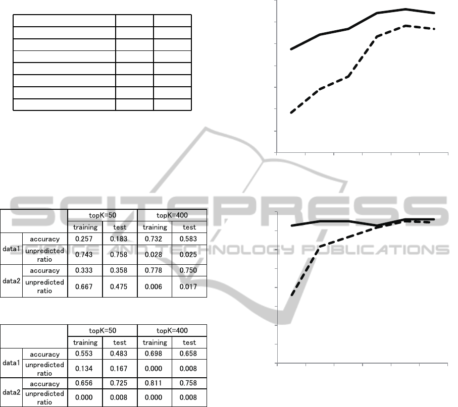
Table 4: Best performance of each method for data2.
CACP CAEP
accuracy 0.758 0.750
precision for pos class 0.767 0.792
precision for neg class 0.763 0.738
recall for pos class 0.767 0.700
recall for neg class 0.750 0.800
F
1
score for pos class 0.767 0.743
F
1
score for neg class 0.756 0.768
Tables 3 and 4 give the best results regarding
the accuracy for each data set, which occurs when
topK = 400 for both methods and both data sets. For
data1, CACP outperforms CAEP with regard to accu-
racy and F
1
score. For data2, CACP has a slightly bet-
ter accuracy and F
1
score for the pos class, however,
and CAEP has a better F
1
score for the neg class.
Figure 5: Results of CAEP.
Figure 6: Results of CACP.
Figure 5 and 6 illustrate training and test results
regarding accuracy and unpredicted ratio for CAEP
and CACP. Although at topK = 400, the results are
similar, at topK = 50, CACP significantly outper-
forms CAEP. The reason for this is the unpredicted
ratio. It means that CAEP cannot make a classifica-
tion model to cover most transactions at topK = 50.
However, CACP is able to do so.
Figures 7 and 8 illustrate the relationship between
topK and accuracy. In these figures, accuracy denotes
test results for each method. For data1, both method
cannot build an efficient model at small topK. How-
ever, CACP can make a good model at topK = 300,
because the unpredicted ratio of CACP is small. For
data2, at topK = 300, the performance is similar for
both methods, but at topK = 50 and 100, the gap be-
tween the performances is large.
0.000
0.100
0.200
0.300
0.400
0.500
0.600
0.700
50 100 200 300 400 500
CACP
(our proposed method)
CAEP(existing method)
Number of topK patterns
Accuuracy
Figure 7: Effect on topK in case data1.
0.000
0.100
0.200
0.300
0.400
0.500
0.600
0.700
0.800
50 100 200 300 400 500
CACP(our proposed method)
CAEP(existing method)
Number of topK patterns
Accuuracy
Figure 8: Effect on topK in case data2.
Figures 9 and 10 illustrate scatter plots of emerg-
ing patterns and contrast patterns for both classes at
topK = 50 and 400, respectively. In the figure, ”cp”
and ”ep” denote contrast patterns and emerging pat-
terns. In Figure 9, we can see that CAEP build its
model using emerging patterns located only at the
lower left corner, because top the 50 emerging pat-
terns are located only in that area. On the other
hand, CACP may use contrast patterns located within
a broader area. In particular, contrast patterns located
at the upper right corner cover more frequently oc-
curring transactions, because the patterns located here
have a larger support value. In Figure 10, CAEP can
use emerging patterns located within broader area,
however compared to CACP, it is still limited.
The performance gap between CAEP and CACP
is caused by such a pattern usages. From our test re-
sults, it can be seen that CACP performs well on the
ICEIS2013-15thInternationalConferenceonEnterpriseInformationSystems
338

0
0.1
0.2
0.3
0.4
0.5
0.6
0.7
0 0.1 0.2 0.3 0.4 0.5 0.6 0.7
cp for neg class
cp for pos class
ep for neg class
ep for pos class
Support value for neg class
Support value for pos class
Figure 9: Scatter plot of patterns topK = 50.
0
0.1
0.2
0.3
0.4
0.5
0.6
0.7
0 0.1 0.2 0.3 0.4 0.5 0.6 0.7
cp for neg class
cp for pos class
ep for neg class
ep for pos class
Support value for pos class
Support value for neg class
Figure 10: Scatter plot of patterns at topK = 400.
data. It is expected that for other data sets, CACP will
also give good results.
5 CONCLUSIONS
In this paper, we proposed a new classification model
called CACP, which uses contrast patterns to address
existing problems. Computational experiments using
real business data showed that our method is better
than the existing method. In particular, our method is
advantageous in that it constructs a sufficient model
using only a small number of contrast patterns. For
real, larger-size, and difficult problems, we expect
that our method will have further advantage.
REFERENCES
Bay, S. D. and Pazzani, M. J. (1999). Detecting change in
categorical data: Mining contrast sets. In In Proceed-
ings of the Fifth International Conference on Knowl-
edge Discovery and Data Mining, pages 302–306.
ACM Press.
Dong, G., Zhang, X., Wong, L., and Li, J. (1999). Caep:
Classification by aggregating emerging patterns. In
Arikawa, S. and Furukawa, K., editors, Discovery Sci-
ence, volume 1721 of Lecture Notes in Computer Sci-
ence, pages 30–42. Springer Berlin Heidelberg.
Morita, H. and Hamuro, Y. (2013). A classification model
using emerging patterns incorporating item taxonomy.
In Gaol, F. L., editor, Recent Progress in Data Engi-
neering and Internet Technology, volume 156 of Lec-
ture Notes in Electrical Engineering, pages 187–192.
Springer Berlin Heidelberg.
Takizawa, A., Koo, W., and Katoh, N. (2010). Discovering
distinctive spatial patterns of snatch theft in kyoto city
with caep. Journal of Asian Architecture and Building
Engineering, 9(1):103–110.
Uno, T., Asai, T., Uchida, Y., and Arimura, H. (2003).
Lcm: An efficient algorithm for enumerating frequent
closed item sets. In In Proceedings of Workshop on
Frequent itemset Mining Implementations (FIMI03).
ClassificationModelusingContrastPatterns
339