
Some Synchronization Issues in OSPF Routing
Anne Bouillard
1
, Claude Jard
2
and Aurore Junier
3
1
ENS/INRIA, Paris, France
2
LINA, University of Nantes, Nantes, France
3
INRIA, Rennes, France
Keywords:
OSPF Routing, Synchronization, Simulation, Time Petri Nets.
Abstract:
A routing protocol such as OSPF has a cyclic behavior to regularly update its view of the network topology. Its
behavior is divided into periods. Each period produces a flood of network information messages. We observe a
regular activity in terms of messages exchanges and filling of receive buffers in routers. This article examines
the consequences of possible overlap of activity between periods, leading to a buffer overflow. OSPF allows
“out of sync" flows by considering an initial delay (phase). We study the optimum calculation of these offsets
to reduce the load, while maintaining a short period to ensure a protocol reactive to topology changes. Such
studies are conducted using a simulated Petri net model. A heuristic for determining initial delays is proposed.
A core network in Germany serves as illustration.
1 INTRODUCTION
Routing protocols generally work in a dynamic en-
vironment where they have to constantly monitor
changes. This function is implemented locally in
routers by a programming loop that generates regu-
lar behaviors. Open Shortest Path First (OSPF) pro-
tocol (Moy, 1998) is an interesting example, widely
used in networks. OSPF is a link-state protocol that
performs internal IP routing. This protocol regularly
fills the network with messages “hello” to monitor the
changes of network topology and messages “link state
advertisements” (LSA) to update the table of shortest
paths in each router.
A lot of work (Francois et al., 2005; Basu and
Riecke, 2001) has been devoted to stability issues.
The stability is required if there is a change in the
network state (e.g., a link goes down), all the nodes
in the network are guaranteed to converge to the new
network topology in finite time (in the absence of
any other events). The question is difficult when the
change is determined as a result of a bottleneck in
a router (as possible in the OPSF-TE (Katz et al.,
2003)). If the response to a congestion is the exchange
of additional messages, the situation may become
critical. But it has been proved (Basu and Riecke,
2001) that OSPF-TE is rather robust in that matter.
In this article we look at a related problem which
is to focus on the possibilities of congestion of the
input buffers of routers due to LSA traffic. Indeed,
we believe that there are situations where the cycli-
cal behavior of routers may cause harmful timings in
which incoming messages collide in a very short time
in front of routers.
In current implementations, the refresh cycle is
very slow and congestion is unlikely in view of the
routers’ response time. Nevertheless, we address the
question to increase the refresh rate to ensure better
responsiveness to changes. This article shows a pos-
sibility of divergence, and discusses the possibilities
of avoiding harmful synchronization by adjusting the
phase shift of cyclical behavior.
The approach is as follows. We modeled LSAs ex-
changes using TimePetri Nets (in a fairly abstract rep-
resentation). This model was simulated for a topology
of 17 nodes representing the heart of an existing net-
work in Germany (data provided by Alcatel). We then
demonstrated the possibility of accumulation of mes-
sages for well-chosen parameter values. Accumula-
tion is due to a possible overlap of refresh phases in
terms of messages. To validate this model, and thus
the reality of the observed phenomenon, we repro-
duced it on a network emulator available from Alca-
tel. Curves could indeed be replicated. Parameter val-
ues were different, but it was difficult to believe that
the model scaled with respect to the rough abstraction
performed. Once the problem identified, the question
is then to try to solve it by computing optimum initial
5
Bouillard A., Jard C. and Junier A..
Some Synchronization Issues in OSPF Routing.
DOI: 10.5220/0004506800050014
In Proceedings of the 4th International Conference on Data Communication Networking, 10th International Conference on e-Business and 4th
International Conference on Optical Communication Systems (DCNET-2013), pages 5-14
ISBN: 978-989-8565-72-3
Copyright
c
2013 SCITEPRESS (Science and Technology Publications, Lda.)

delays. Such a computation can be performed using
linear integer programming on a simplified graphical
model. We will show using simulation that the com-
puted values are relevant to avoid message accumula-
tion in front of routers.
The rest of the paper is organized as follows: we
first present in section 2 the modeling of the LSA
flooding process and its validation. In section 3, simu-
lation shows a possible overload of buffers depending
on the refresh period. Then, in section 4, we study a
possible adjustment of the initial delays, which aims
at minimizing the overload. We show how to compute
these delays. The impact is then demonstrated using
simulation.
2 TPN MODELING OF THE LSA
FLOODING PROCESS
2.1 LSA Flooding Process
The network is represented by a directed graph G =
(V,E), whereV is a finite set of n vertices (the routers)
and E is a binary relation on V to represent the links.
The i
th
router is denoted by R
i
. The set V (R
i
) denotes
the set of neighbors of R
i
, of cardinality |V (R
i
)|. To
help the reader Table 1 gives the list of the main nota-
tions introduced in this paper.
The LSA flooding occurs periodically every T
r
seconds (30 minutes in the standard). Thus, the LSA
flooding process starts at time kT
r
, ∀k ∈ N.
The LSA of a router R
i
records the content of its
database. Then, R
i
shares this LSA (denoted LSA
i
)
with its neighbors to communicate its view of the net-
work at the beginning of each period. The router R
i
sends LSA
i
after an initial delay d
i
. More precisely,
R
i
sends LSA
i
at d
i
+ kT
r
, ∀k ∈ N. Suppose that a
router R
j
receives LSA
i
and that it starts processing it
at time t. Then, R
j
ended the processing of LSA
i
at
time t + T
p
, where T
p
is the time needed by any router
to process an LSA or an acknowledgment(Ack). Dur-
ing this processing, R
j
updates its database and sends
a new LSA to its other neighbors if some new infor-
mation is learned. Consequently, R
j
could send a new
LSA at time t + T
p
, and its neighbors will receive it at
time t + T
p
+ T
t
, where T
t
represents the time to send
a message.
Note that any information received by R
j
can be
taken into account if some properties are satisfied.
The most important one is the age of the LSA. An
LSA that is too old is simply ignored. In all cases, at
time t + T
p
, R
j
sends an Ack to R
i
. The objective is
to inform R
i
that LSA
i
has been correctly received. In
parallel, R
i
waits for an Ack from all of its neighbors
before a given time. If an Ack is not received before
the end of this time, R
i
sends LSA
i
again until an Ack
is properly received.
The LSA flooding process ends when every router
has synchronized to the same database.
2.2 The Simulation Model
Time Petri Net (TPN) (Jard and Roux, 2010) is an
efficient tool to model discrete-event systems and to
capture the inherent concurrency of complex systems.
In the classical definition, transitions are fired over an
interval of time. Here, transitions are fired at a fixed
time. This assumption is justified by observations of
actual OSPF traces whose data processing time does
not vary that much. In our case, the formal definition
of TPN is the following:
Definition 2.1 (Time Petri Net). A Time Petri Net
(TPN) is a tuple (P,T,B,F,M
0
,ϕ) where
• P is a finite non-empty set of places;
• T is a finite non-empty set of transitions;
• B : P×T → N is the backward incidence function;
• F : T × P → N is the forward incidence function;
• M
0
: P → N is the initial marking function;
• ϕ : T → N is the temporal mapping of transitions.
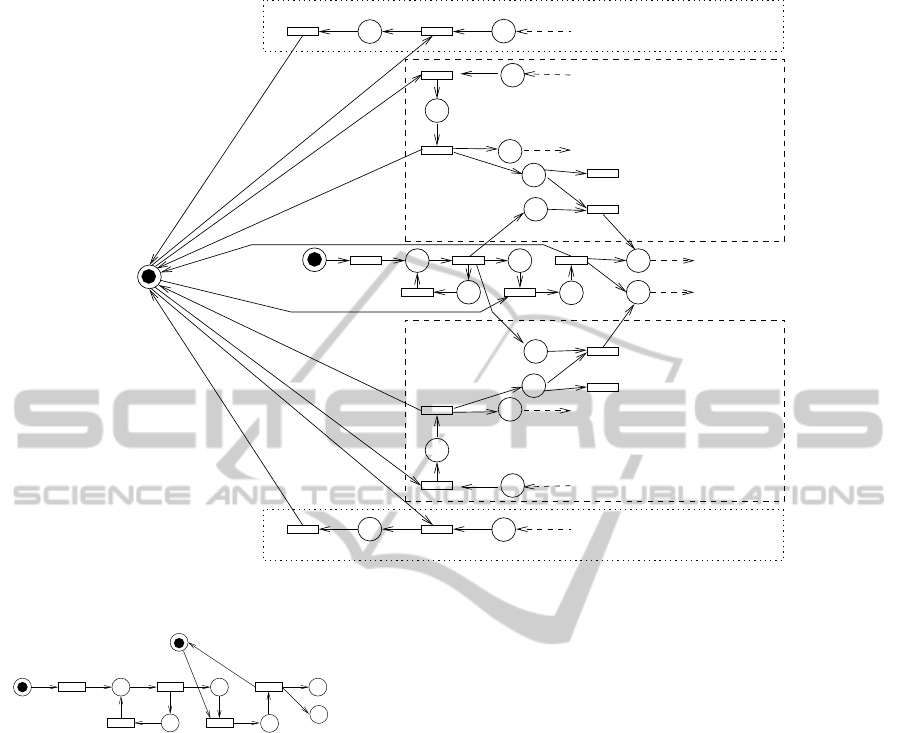
The remainder of this part is devoted to the con-
struction of the TPN that models message exchanges
of the LSA flooding process. The objective is to
model and observe the dynamic behavior of a given
network.
Router Modeling The TPN that models the behav-
ior of the LSA flooding process in a router R
i
needs
three timers: d
i
, T
r
and T
p
. Their functions are:
creating LSA
i
, managing a message received and re-
transmitting a received LSA when needed. Messages
are processed one by one. The following paragraphs
present each functional part of the TPN that models a
router.
• Place Processor. Initially this place contains
one token, representing the processing resource of a
router that is used to process LSAs and Acks. This
place mimics the queuing mechanism of R
i
and guar-
anties that only one message is processed at once. For
each different kind of messages (LSA
i
and Ack) the
processing mechanism is the following: an instanta-
neous transition is fired, to reserve the resource of R
i
.
Note that it can only be fired if a message is wait-
ing. Then the successor transition with timing T
p
can
be fired, modeling the processing time of the router,
and Processor becomes marked again, enabling the
processing of a new message.
DCNET2013-InternationalConferenceonDataCommunicationNetworking
6
ACKs arrivals from a neighbor
LSAs arrivals from a neighbor
Acks sendings to the sender
ACKs arrivals from a neighbor
LSAs arrivals from a neighbor
Acks sendings to the sender
Start
i
d
i
T
r
0
T
p
LSAsend
i→k
T
p
LSArec
j→i
ACKrec
j→i
ACKsend
i→ j
0
0
T
p
0
0
Retransmission
Destruction
bound
T
p
LSArec
k→i
ACKrec
k→i
ACKsend
i→k
0
0
T
p
0
0
Retransmission
Destruction
bound
b
i
0
b
i
Processor
LSAsend
i→ j
Figure 2: TPN of a router R
i
that has two neighbors, R
j
and R
k
.
p
3
LSAsend
i→k
p
5
T
p
t
5
LSAsend
i→ j
t
3
p
2
0t
2
t
4
0
T
r
p
4
Processor
Start
i
t
1
d
i
Figure 1: Part of TPN that creates the LSA of a router R
i
.
• Creation of LSA. Figure 1 represents the part
of the TPN that creates LSA
i
s at time d
i
+ kT
r
, for
k ∈ N in router R
i
. Initially Start
i
contains one to-
ken, t
1
fires at time d
i
and a token appears in p
2
at time d
i
for the first time. Afterward, the cycle
p
2
,t
2
, p
3
,t
3
generates a token in p
4
at times d
i
+ kT
r
,
k ∈ N. Those token will be processed using the mech-
anism described above, generating tokens in places
LSAsend
i→ j
, R
j
∈ V (R
i
).
• Reception of an Ack (dotted rectangles on Fig-
ure 2) A token in ACKrec
j→i
represents this event.
It is processed using the mechanism described above
and does not generate any new message.
• Reception of an LSA from a neighbor (dashed
rectangles in Figure 2). A token in place LSArec
j→i
represents this event. It is processed using the mech-
anism described above and generate an Ack, that is
sent to the sender. It can also possibly generate an
LSA message that will be retransmitted to its other
neighbors (transition Retransmission). Otherwise, the
token is destroyed (transition Destruction). In the
flooding mechanism, an LSA
j
is retransmitted only
if it is received for the first time during one flooding
period. That way, the LSA flooding process ensures
that every router converges to the same database be-
fore the end of every period. To model this, we bound
the number of retransmissions per period (for R
i
, the
number of retransmissions of an LSA received from
R
j
is b
i
, that is modeled by placing b
i
tokens in each
place bound of R
i
at the beginning of each period).
The tokens are inserted in these places by weighted
arcs between t
2
and each place bound.
• Global TPN Figure 2 represents the behavior
for one router. Such a net is built for each router. Fi-
nally, place LSAsend
i→ j
(resp. ACKsend
i→ j
) is con-
nected to place LSArec
i→ j
(resp. ACKrec
i→ j
) by in-
serting a transition LSA
i→ j
(resp. ACK
i→ j
) with firing
time T
t
between them.
2.3 Model Validation
We performed our experimentations on the 17-node
German telecommunication network represented in
Figure 3. This article focuses on the study of router R
8
that has the largest number of neighbors (|V (R
8
)| =
6).
SomeSynchronizationIssuesinOSPFRouting
7

R
5
R
4
R
10
R
3
R
14
R
2
R
7
R
1
R
8
R
12
R
9
R
16
R
17
R
13
R
15
R
6
R
11
Figure 3: German telecommunication network.
The arrivals of LSAs and Acks in the actual net-
work are captured by an emulation using the Quagga
Routing Software Suite (Ishiguro, 2012), where each
node is set from an Ubuntu Linux machine that hosts
a running instance of the Quagga Routing Software
Suite. Figure 4 represents the arrival of messages in
R
8
by the emulation of the LSA flooding on the Ger-
man topology during 8000s with T
r
= 1800s.
0
50
100
150
200
250
300
350
0 1000 2000 3000 4000 5000 6000 7000 8000
umber of messages arrived
time(s)
r
r
r
r
r
r
r
r
r
r
r
r
r
r
r
r
r
r
r
r
r
r
r
r
r
r
r
r
r
r
r
r
r
r
r
r
r
r
r
r
r
r
r
r
r
r
r
r
r
r
r
r
r
r
r
r
r
r
r
r
r
r
r
r
r
r
r
r
r
r
r
r
r
r
r
r
r
r
r
r
r
r
r
r
r
r
r
r
r
r
r
r
r
r
r
r
r
r
r
r
r
r
r
r
r
r
r
r
r
r
r
r
r
r
r
r
r
r
r
r
r
r
r
r
r
r
r
r
r
r
r
r
r
r
r
r
r
r
r
r
r
r
r
r
r
r
r
r
r
r
r
r
r
r
r
r
r
r
r
r
r
r
r
r
r
r
r
r
r
r
r
r
r
r
r
r
r
r
r
r
r
r
r
r
r
r
r
r
r
r
r
r
r
r
r
r
r
r
r
r
r
r
r
r
r
r
r
r
r
r
r
r
r
r
r
r
r
r
r
r
r
r
r
r
r
r
r
r
r
r
r
r
r
r
r
r
r
r
r
r
r
r
r
r
r
r
r
r
r
r
r
r
r
r
r
r
r
r
r
r
r
r
r
r
r
r
r
r
r
r
r
r
r
r
r
r
r
r
r
r
r
r
r
r
r
r
r
r
r
r
r
r
r
r
r
r
r
r
r
r
r
Figure 4: Emulation of the arrivals to R
8
.
During the emulation, the processors of routers
are parametrized with a 900 MHz CPU, and the mean
size of an LSA (resp. an Ack) is 96 bytes (resp. 63
bytes). The processing time of an LSA (resp. an Ack)
is approximately 0.8 µs (resp. 0.5 µs). The transmis-
sion time of an LSA (resp. an Ack) in 96 ms (resp. 64
ms).
Unfortunately, these parameters can not be used
directly to parametrize the TPN, as the TPN only
represents the behavior of the LSA flooding process.
However,an actual router is much more loaded. Thus,
T
p
and T
t
must be adjusted to include the whole load
of the router.
The simulations presented in this article are pro-
duced by the software Renew (see (Kummer et al.,
2003)) which can simulate Time Petri Nets. Note
that the TPN are automatically generated (the TPN
that models the German Telecommunication network
is not represented here due to its size). Figure 5 rep-
resents the simulation of message arrivals using the
TPN where T
r
= 1800s, T
p
= 15s, T
t
= 30s. To corre-
spond to the sendings emulated in Figure 4 the num-
ber of LSAs retransmitted per neighbour during a pe-
riod is b
i
= ⌈
(n−1)
4|V (R
i
)|
⌉.
One can observe that Figure 4 and 5 are quite sim-
ilar: the parameters chosen as above are defined to
represent the actual behavior of an LSA flooding pro-
0
50
100
150
200
250
300
350
0 1000 2000 3000 4000 5000 6000 7000 8000
Number of messages arrived
time(s)
r
r
r
r
r
r
r
r
r
r
r
r
r
r
r
r
r
r
r
r
r
r
r
r
r
r
r
r
r
r
r
r
r
r
r
r
r
r
r
r
r
r
r
r
r
r
r
r
r
r
r
r
r
r
r
r
r
r
r
r
r
r
r
r
r
r
r
r
r
r
r
r
r
r
r
r
r
r
r
r
r
r
r
r
r
r
r
r
r
r
r
r
r
r
r
r
r
r
r
r
r
r
r
r
r
r
r
r
r
r
r
r
r
r
r
r
r
r
r
r
r
r
r
r
r
r
r
r
r
r
r
r
r
r
r
r
r
r
r
r
r
r
r
r
r
r
r
r
r
r
r
r
r
r
r
r
r
r
r
r
r
r
r
r
r
r
r
r
r
r
r
r
r
r
r
r
r
r
r
r
r
r
r
r
r
r
r
r
r
r
r
r
r
r
r
r
r
r
r
r
r
r
r
r
r
r
r
r
r
r
r
r
r
r
r
r
r
r
r
r
r
r
r
r
r
r
r
r
r
r
r
r
r
r
r
r
r
r
r
r
r
r
r
r
r
r
r
r
r
r
r
r
r
r
r
r
r
r
r
r
r
r
r
r
r
r
r
r
r
r
r
r
r
r
r
r
r
r
r
r
r
r
r
r
r
r
r
r
r
r
r
r
r
r
r
r
r
r
r
r
r
r
r
r
Figure 5: Message arrivals to R
8
with T
r
= 1800s.
cess. The two curves are both composed of periods
that last 1800s. They show on each period a burst of
message arrivals that lasts approximately 800s, then
message arrivals stop until the next period. We there-
fore conclude that our abstract model correctly cap-
tures the phenomenon of LSA flooding.
From now on we fix the parameters ((b
i
)
i∈{1,...,n}
,
T
p
, T
t
and T
r
) as defined above.
3 STUDY OF PERIOD LENGTH
We study here the effect of the period length T
r
on
both message arrivals and queue length. We first dis-
cuss the normal case where T
r
= 1800s. Then, we
present a congested case where T
r
= 514s. Finally,
we observe a limit case where T
r
= 1000s.
3.1 Low Traffic Case
Figure 6 represents the simulated queue length of R
8
during 10
5
s (approx. 1 day), where T
r
= 1800s. One
can observe a lot of fluctuations. At the beginning
of each period R
8
receives and processes messages.
However, the number of messages that are received
is much larger than those which are processed. Con-
sequently, the queue length increases. Afterward, the
sendings stop, and R
i
keeps processing messages. The
queue length decreases.
0
5
10
15
20
25
30
35
40
0 10000 20000 30000 40000 50000 60000 70000 80000 90000 100000
Queue length
time(s)
Figure 6: Buffer length of R
8
with T
r
= 1800s.
DCNET2013-InternationalConferenceonDataCommunicationNetworking
8
3.2 Congested Case
Figure 7 represents the message arrivals in R
8
during
8000s, and Figure 8 the queue length of R
8
during
10
5
s, where T
r
= 514s. One can observe that mes-
sages arrive continuously on router R
8
. Then, R
8
is
never idle and never empties its queue. Consequently
the queue length permanently increases.
0
100
200
300
400
500
600
700
800
900
1000
0 1000 2000 3000 4000 5000 6000 7000 8000
Number of messages arrived
time(s)
rr
r
r
rr
r
r
rr
r
rr
r
r
rr
r
r
rr
r
rr
r
r
rr
r
r
rr
r
r
rr
r
rr
r
r
rr
r
r
rr
r
rr
r
r
rr
r
r
rr
r
rr
r
r
rr
r
r
rr
r
rr
r
r
rr
r
r
rr
r
r
rr
r
rr
r
r
rr
r
r
rr
r
rr
r
r
rr
r
r
rr
r
rr
r
r
rr
r
r
rr
r
rr
r
r
rr
r
r
rr
r
rr
r
r
rr
r
r
rr
r
r
rr
r
rr
r
r
rr
r
r
rr
r
rr
r
r
rr
r
r
rr
r
rr
r
r
rr
r
r
rr
r
rr
r
r
rr
r
r
rr
r
r
rr
r
rr
r
r
rr
r
r
rr
r
rr
r
r
rr
r
r
rr
r
rr
r
r
rr
r
r
rr
r
rr
r
r
rr
r
r
rr
r
r
rr
r
rr
r
r
rr
r
r
rr
r
rr
r
r
rr
r
r
rr
r
rr
r
r
rr
r
r
rr
r
rr
r
r
rr
r
r
rr
r
rr
r
r
rr
r
r
rr
r
r
rr
r
rr
r
r
rr
r
r
rr
r
rr
r
r
rr
r
r
rr
r
rr
r
r
rr
r
r
rr
r
rr
r
r
rr
r
r
rr
r
r
rr
r
rr
r
r
rr
r
r
rr
r
rr
r
r
rr
r
r
rr
r
rr
r
r
rr
r
r
rr
r
rr
r
r
rr
r
r
rr
r
rr
r
r
rr
r
r
rr
r
r
rr
r
rr
r
r
rr
r
r
rr
r
rr
r
r
rr
r
r
rr
r
rr
r
r
rr
r
r
rr
r
rr
r
r
rr
r
r
rr
r
r
rr
r
rr
r
r
rr
r
r
rr
r
rr
r
r
rr
r
r
rr
r
rr
r
r
rr
r
r
rr
r
rr
r
r
rr
r
r
rr
r
r
rr
r
rr
r
r
rr
r
r
rr
r
rr
r
r
rr
r
r
rr
r
rr
r
r
rr
r
r
rr
r
rr
r
r
rr
r
r
rr
r
rr
r
r
rr
r
r
rr
r
r
rr
r
rr
r
r
rr
r
r
rr
r
rr
r
r
rr
r
r
rr
r
rr
r
r
rr
r
r
rr
r
rr
r
r
rr
r
r
rr
r
r
rr
r
rr
r
r
rr
r
r
rr
r
rr
r
r
rr
r
r
rr
r
rr
r
r
rr
r
r
rr
r
rr
r
r
rr
r
r
rr
r
rr
r
r
rr
r
r
rr
r
r
rr
r
rr
r
r
rr
r
r
rr
r
rr
r
r
rr
r
r
rr
r
rr
r
r
rr
r
r
rr
r
rr
r
r
rr
r
r
rr
r
r
rr
r
rr
r
r
rr
r
r
rr
r
rr
r
r
rr
r
r
rr
r
rr
r
r
rr
r
r
rr
r
rr
r
r
rr
r
r
rr
r
rr
r
r
rr
r
r
rr
r
r
rr
r
rr
r
r
rr
r
r
rr
r
rr
r
r
rr
r
r
rr
r
rr
r
r
rr
r
r
rr
r
rr
r
r
rr
r
r
rr
r
r
rr
r
rr
r
r
rr
r
r
rr
r
rr
r
r
rr
r
r
rr
r
rr
r
r
rr
r
r
rr
r
rr
r
r
rr
r
r
rr
r
r
rr
r
rr
r
r
rr
r
r
rr
r
rr
r
r
rr
r
r
rr
r
rr
r
r
rr
r
r
rr
r
rr
r
r
rr
r
r
rr
r
rr
r
Figure 7: Message arrivals to R
8
with T
r
= 514s.
0
1000
2000
3000
4000
5000
6000
0 10000 20000 30000 40000 50000 60000 70000 80000
90000
100000
Queue length
time(s)
Figure 8: Buffer size of R
8
with T
r
= 514s.
3.3 Limit Case
Figure 9 represents the message arrivals in R
8
during
8000s, and Figure 10 shows the queue length of router
R
8
during 10
5
s, where T
r
= 1000s. This time, the
sendings of a period are not merged with the sendings
of the next period. Then, each period is long enough
so that R
8
can process messages from its queue be-
fore the beginning of the next one. Figure 10 shows
the fluctuations of the queue length that correspond to
this. However the queue length is not empty at the
end of each period. Consequently, the stability of this
router is not ensured.
3.4 Sufficient Condition for Congestion
Suppose being in the worst case where each router
learns some new information from each router and let
us now focus on the quantity of messages received
during a period.
Theorem 3.1. Let n( j) be the number of messages
received by a router R
j
during a flooding period T
r
.
0
50
100
150
200
250
300
350
400
450
500
0 1000 2000 3000 4000 5000 6000 7000 8000
Number of messages arrived
time(s)
r
r
r
r
r
r
r
r
r
r
r
r
r
r
r
r
r
r
r
r
r
r
r
r
r
r
r
r
r
r
r
r
r
r
r
r
r
r
r
r
r
r
r
r
r
r
r
r
r
r
r
r
r
r
r
r
r
r
r
r
r
r
r
r
r
r
r
r
r
r
r
r
r
r
r
r
r
r
r
r
r
r
r
r
r
r
r
r
r
r
r
r
r
r
r
r
r
r
r
r
r
r
r
r
r
r
r
r
r
r
r
r
r
r
r
r
r
r
r
r
r
r
r
r
r
r
r
r
r
r
r
r
r
r
r
r
r
r
r
r
r
r
r
r
r
r
r
r
r
r
r
r
r
r
r
r
r
r
r
r
r
r
r
r
r
r
r
r
r
r
r
r
r
r
r
r
r
r
r
r
r
r
r
r
r
r
r
r
r
r
r
r
r
r
r
r
r
r
r
r
r
r
r
r
r
r
r
r
r
r
r
r
r
r
r
r
r
r
r
r
r
r
r
r
r
r
r
r
r
r
r
r
r
r
r
r
r
r
r
r
r
r
r
r
r
r
r
r
r
r
r
r
r
r
r
r
r
r
r
r
r
r
r
r
r
r
r
r
r
r
r
r
r
r
r
r
r
r
r
r
r
r
r
r
r
r
r
r
r
r
r
r
r
r
r
r
r
r
r
r
r
r
r
r
r
r
r
r
r
r
r
r
r
r
r
r
r
r
r
r
r
r
r
r
r
r
r
r
r
r
r
r
r
r
r
r
r
r
r
r
r
r
r
r
r
r
r
r
r
r
r
r
r
r
r
r
r
r
r
r
r
r
r
r
r
r
r
r
r
r
r
r
r
r
r
r
r
r
r
r
r
r
r
r
r
r
r
r
r
r
r
r
r
r
r
r
r
r
r
r
r
r
r
r
r
r
r
r
r
r
r
r
r
r
r
r
r
r
r
r
r
r
r
r
r
r
r
r
r
r
r
r
r
r
r
r
r
r
r
r
r
r
r
r
r
r
r
r
r
r
r
r
r
r
r
r
r
r
r
r
r
r
r
r
r
r
r
r
r
r
r
r
r
r
r
r
r
r
r
r
r
r
r
r
r
r
r
r
r
r
r
r
Figure 9: Message arrivals to R
8
with T
r
= 1000s.
0
5
10
15
20
25
30
35
0 10000 20000 30000 40000 50000 60000 70000 80000
90000
100000
Queue length
time(s)
Figure 10: Buffer length of R
8
with T
r
= 1000s.
Then
n( j) > n(|V (R
j
)|).
Proof. Let us first focus on the case of networks with
a tree topology. In this case, we show that the above
inequality is in fact an equality. Two kinds of mes-
sages can be received: LSAs and Acks. Let us first
count the number of messages received by router R
j
concerning the flooding from router R
i
. Consider R
i
as the root of the tree, R
j
can receive LSA
i
from its fa-
ther only: R
j
will receiveone and only once LSA
i
. Af-
terward R
j
sends LSA
i
to its children and will receive
an Ack (as illustrated in Figure 11). As a consequence,
the number of messages received for the flooding of
LSA
i
is the number of neighbors of R
j
. Consider the
flooding of LSA
j
. The router R
j
sends the LSA to its
neighbors and will receive an Ack from them. Glob-
LSA
i
sent at step j
1
1
j
ack sent in response to LSA
i
received
2
R
j
R
i
1
2
2
2
2
Figure 11: Flooding of LSA
i
: LSA and ACKs transmissions
in a tree topology.
SomeSynchronizationIssuesinOSPFRouting
9

ally, R
j
will then receive exactly n(|V (R
j
)|) mes-
sages.
For networks with a general topology, one can ob-
serve that the flooding of LSA
i
defines a spanning tree
of the graph: (R
j
,R
k
) is an edge of the spanning tree
if R
k
first received LSA
i
from R
j
. Then for the flood-
ing of LSA
i
, R
j
receives at least the messages it would
receivedif the topology were the spanning tree, which
gives the desired inequality.
The number of messages processed by router R
j
during a flooding period is 1+ n( j): it processes the
received messages plus LSA
j
. Define N( j) the num-
ber of messages processed during a flooding period
by R
j
, we have
N(j) = n(|V (R
j
)|) + 1.
If a router can not process every message of its
buffer before the end of each period a congestion oc-
curs. Also, given the minimal bound of Theorem 3.1
the congestion is ensured by the following threshold
on T
r
.
Lemma 3.2. If T
r
< T
p
N(j) then the queue length of
R
j
tends to infinity.
Proof. The proof is straightforward from Theo-
rem 3.1.
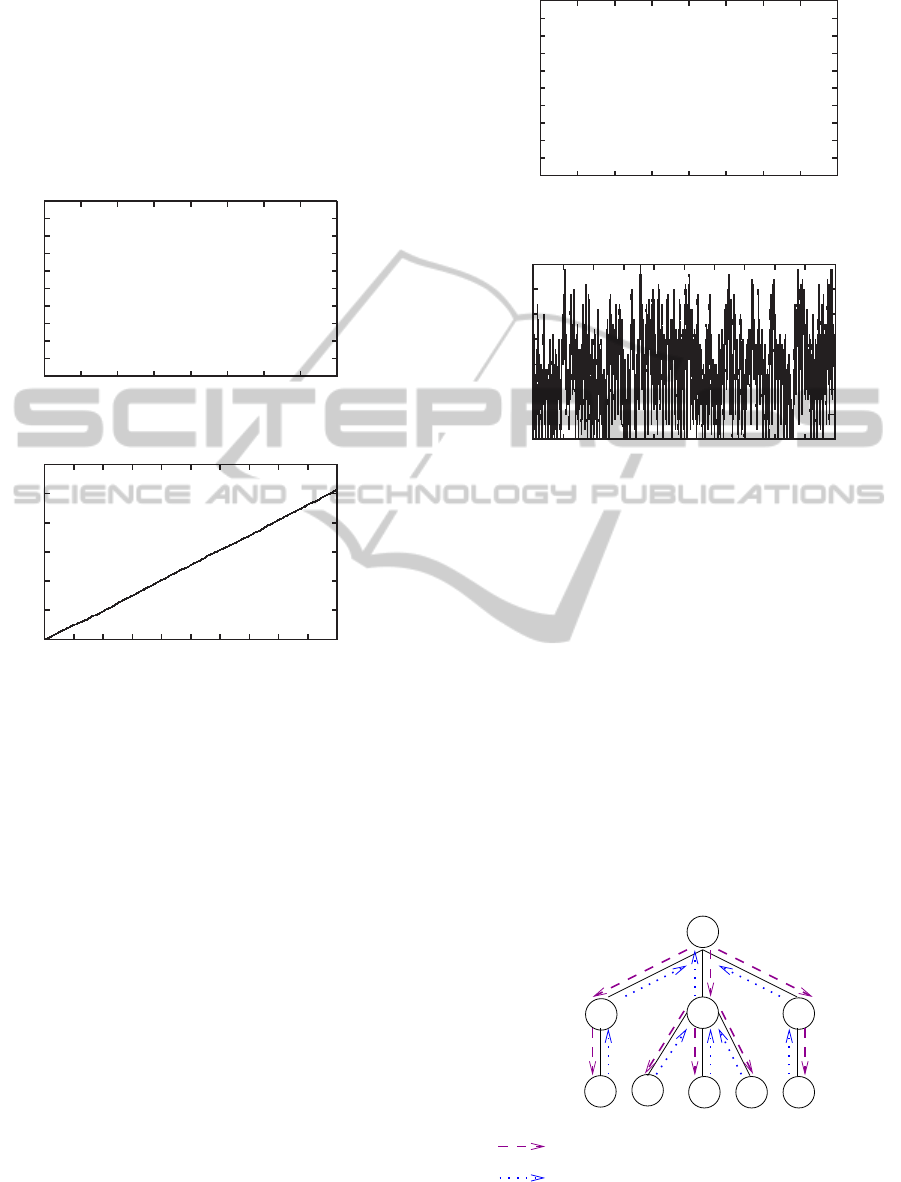
Example 3.3 (Simulation of TPN by Renew soft-
ware). Consider the tree topology network of Fig-
ure 11. Theorem 3.1 ensures that the number of mes-
sages received by R
j
(|V (R
j
)| = 4) is N(j) = 9× 4+
1 = 37. Therefore, if T
p
is set to 15 s in the TPN, if
T
r
< 15 × 37 = 555 s the network is congested. Sim-
ulation of the TPN, representing this topology, with
T
p
= 15s, T
r
= 554s, T
t
= 30s has been made during
4.10
5
s to illustrate this result. The evolution of the
queue length of router R
j
is shown in Figure 12. The
queue length of R
j
clearly increases during the simu-
lation, showing that the network is congested. Finally,
as the simulation has been made with the largest pe-
riod length that ensures congestion, during each pe-
riod, R
j
has enough time to process many messages
from his queue. Consequently, one can observe that
the queue length varies a lot.
4 COMPUTING OPTIMUM
INITIAL DELAYS
In Section 2.2, we emulated the flooding phenomenon
of the OSFP protocol using Time Petri nets. The ini-
tial idea was to consider initial delays for each router
0
10
20
30
40
50
60
70
80
0 50000 100000 150000 200000 250000 300000 350000 400000
Queue length
time(s)
Figure 12: Queue length of R
3
with T
r
= 554s of tree topol-
ogy.
as parameters. The question is then to infer con-
straints on these parameters that ensure a minimum
size of the input buffers. Even if this kind of question
can be theoretically solved using symbolic model-
checking (Lime et al., 2009), the computation com-
plexity is high. The state of the art of the current ex-
isting tools did not allow us to automatically produce
such symbolic constraints.
In order to compute initial delays, we adopt the
following method. We only take into account the mes-
sage contributing to the flooding mechanism: when
an LSA message concerning router R
j
is received at
router R
i
, it is forwarded only if it is received for the
first time. Then, we will model neither the LSA mes-
sages that are not the first to be received at a node, nor
the Acknowledgments.
4.1 Constraints Modeling
Our goal is to perform the floodings as closed as pos-
sible while interacting as little as possible. We say
that two floodings do not interact if, for each router,
the first LSA received from those two floodings in that
router are not queued at the same time.
More formally, we consider a graph G = (V, E),
where V = {R
1
,... ,R
n
} is the set of routers and
E ⊆ V ×V is the set of links between the routers. If
(R
i
,R
j
) ∈ E, then τ
i, j
denotes the transmission time
between R
i
and R
j
, and τ
i, j
= ∞ if (R
i
,R
j
) /∈ E. The
sojourn time of a message in R
i
, between its recep-
tion and its forwarding, belongs to the interval [δ
i
,∆
i
[.
This time also holds for the source of messages.
Let us first compute the intervals of time I
i, j
when the first LSA originating from R
i
is received
in R
j
if the flooding starts at time 0. If i = j, then
I
i,i
= [0,0], and otherwise, we have I
i, j
= [α
i, j
,β
i, j
[
where α
i, j
= min
k∈{1,...,n}
α
i,k
+ δ
k
+ τ
k, j
and β
i, j
=
min
k∈{1,...,n}
β
i,k
+ ∆
k
+ τ
k, j
.
The quantities α
i,k
+ δ
k
and β
i,k
+ ∆
k
respectively
represent the minimal and the maximal departure
times from R
k
.
DCNET2013-InternationalConferenceonDataCommunicationNetworking
10

For the computation of both α
i, j
and β
i, j
, we recog-
nize the computation of a shortest path in a graph with
respective edge lengths (δ
i
+ τ
i, j
) and (∆
i
+ τ
i, j
). Let
α = (α
i, j
) and β = (β
i, j
) the matrices of the shortest-
paths. They can, for example, be computed using the
Floyd-Warshall algorithm. Now, the messages origi-
nating from R
i
are present in R
j
during an interval of
time included in [α
i, j
,β
i, j
+ ∆
j
[= [α
i, j
,γ
i, j
[. We de-
note by D
i, j
this interval and D the matrix of these
intervals.
Example 4.1 (Sojourn times in the routers).
R
1
R
3
R
4
R
2
[δ
1
, ∆
1
[= [1, 2[
[δ
4
, ∆
4
[= [2, 3[
[δ
2
, ∆
2
[= [1, 3[
1
2
5
2
[δ
3
, ∆
3
[= [1, 2[
Figure 13: Example of a toy topology.
Figure 13 represents a toy topology with 4 vertices.
Matrix D is then:
D =
[0,2[ [2,6[ [5,9[ [8,14[
[2,6[ [0,3[ [3,7[ [6,12[
[5,9[ [3,7[ [0,2[ [3,7[
[9,14[ [7, 12[ [4,7[ [0,3[
.
Now, if the flooding from server R
i
starts at time
d
i
, its first LSA received by R
j
is present in that server
at most in the interval d
i
+ D
i, j
= [d
i
+ α
i, j
,d
i
+ γ
i, j
].
Then, in order to have no interference between
the floodings in router R
j
, the family of intervals
(d
i
+ D
i, j
)
i∈{1,...,n}
must be two-by-two disjoint, and
to have no interference at all, the following condition
must hold:
∀i, j,k ∈ {1, . ..,n}, i 6= k ⇒ d
i
+ D
i, j
∩ d
k
+ D
k, j
=
/
0,
that is,
∀i, j, k ∈ {1,. ..,n}, i 6= k ⇒
d
i
+ γ
i, j
≤ d
k
+ α
k, j
or
d
k
+ γ
k, j
≤ d
i
+ α
i, j
.
For each triple (i, j,k), the two constraints above are
exclusive: as γ
i, j
> α
i, j
, if one holds, necessarily, the
other one does not hold.
Now, if we don’t consider the first flooding from
each router only, we have to study the interferences
between the first and second flooding from each
router (if there is no interference between those two
sets of flooding, then there will be no interference at
all).
If the flooding period is T, then the constraints
must then be transform in
∀i, j,k ∈ {1, ...,n},
d
i
+ γ
i, j
≤ d
k
+ α
k, j
or
d
k
+ γ
k, j
≤ d
i
+ α
i, j
and
d
k
+ γ
k, j
≤ d
i
+ T + α
i, j
and
d
i
+ γ
i, j
≤ d
k
+ T + α
k, j
(1)
The two cases are illustrated on Figure 14. Note
that, depending on which of the two first constraint
is satisfied, one of the two last inequalities is trivially
satisfied.
d
′
k
+ D
k, j
d
′
k
+ T + D
k, j
d
k
+ D
k, j
d
k
+ T + D
k, j
d
i
+ D
i, j
d
i
+ T + D
i, j
d
′
i
+ T + D
i, j
d
′
i
+ D
i, j
Figure 14: Different possibilities for the constraints. In the
first case, d
i
+D
i, j
is before d
k
+D
k, j
and in the second case,
d
′
k
+ D
k, j
is before d
′
i
+ D
i, j
, but in both cases, d
k
+ D
k, j
is
before d
i
+ T + D
i, j
and d
i
+ D
i, j
is before d
k
+ T +D
k, j
The problem we want to solve is then to find
(d
i
)
i∈{1,...,n}
such that all the constraints are satisfied
and T is minimized.
Theorem 4.2. Given (α
i, j
)
i, j∈{1,...,n}
, (γ
i, j
)
i, j∈{1,...,n}
and T, the problem of finding (d
i
)
i∈{1,...,n}
satisfying
the constraints of Equation (1) is NP-complete.
Proof. The problem is trivially in NP as for any as-
signment of (d
i
) and period T, it is possible to check
in polynomial time if the constraints are satisfied
(there are O(n
3
) constraints).
Now, to show that the problem is NP-hard, we re-
duce the salesman problem with triangular inequality
to that problem.
Suppose a complete weighted graph, with posi-
tive weights of the edges w(u, v), satisfying the tri-
angular inequality: for all vertices u, v, x, w(u,x) +
w(x,v) ≤ w(u,v). Set γ
i, j
= max
k∈{1,...,n}
w(k,i) and
α
i, j
= γ
k, j
− w(i,k).
This assignment of the variables is made in such a
way that if for some j, d
i
− d
k
≥ γ
k, j
− α
i, j
, then this
holds for all j, as γ
k, j
− α
i, j
= w
i,k
.
Now, let (d
i
) and T be a solution of our problem.
There is a Hamiltonian cycle of weight W ≤ T in the
graph: suppose, without loss of generality that d
1
≤
d
2
≤ · · · ≤ d
n
.
Then, w(1,2) + w(2,3) + ··· + w(n,1) ≤
(d
2
− d
1
) + (d
3
− d
2
) + ··· + (d
1
− d
n
+ T) = T.
Conversely, suppose that there is a Hamiltonian
cycle of weightW, correspondingwithout loss of gen-
erality to the cycle 1, 2, ...,n. Set d
1
= 0 and d
i
=
SomeSynchronizationIssuesinOSPFRouting
11

d
i−1
+ w(i − 1,i). We have for all i, j d
i
every con-
straint is satisfied and T = W is a possible period: if
k > i, d
k
−d
i
= w(i,i+1)+···+w(k− 1,k) ≥ w(i,k).
Moreover, (d
i
+W)−d
k
= w(k,k+1)+···+w(n,i)+
··· + w(i− 1, i) ≥ w(k, i).
Hence, we have a Hamiltonian path of length at
most T if and only if we can find a solution to our
problem with period at most T: the problem is NP-
hard.
4.2 Exact Solution with Linear
Programming
This problem can be solved with a linear program us-
ing both integer and non-integer variables. The trick
is to encode the constraints
d
i
+ γ
i,k
≤ d
k
+ α
k, j
or
d
k
+ γ
k, j
≤ d
i
+ α
i, j
into a linear program, and this is why we introduce
integer variables.
First, this set of constraints can be rewritten in
d
k
− d
i
≥ b
i,k, j
or d
i
− d
k
≥ b
k,i, j
with b
i,k, j
= γ
i, j
− α
k, j
. Set B = max
i, j,k
b
i,k, j
.
Lemma 4.3. There is a solution of this problem where
for all i ∈ {1,...,n}, d
i
∈ [0,nB].
Proof. The assignment d
i
= (i− 1)B is a solution of
the problem. Indeed, ∀i < k, ∀ j ∈ {1,...,n}, d
k
−d
i
=
(k−i)B ≥ B ≥ b
i,k, j
. Moreover, ∀i,k, j, d
k
−d
i
= (n−
k+ i)B ≥ B ≥ b
i,k, j
.
Lemma 4.4. The following sets of constraints are
equivalent.
(i) d
i
,d
k
∈ [0,nB] and (d
k
− d
i
≥ b
i,k, j
or d
i
− d
k
≥
b
k,i, j
)
(ii) d
i
,d
k
∈ [0,nB], q ∈ {0,1} and d
k
− d
i
+ (1 −
q)nB ≥ b
i,k, j
and d
i
− d
k
+ qnB ≥ b
k,i, j
.
Proof. Suppose that the constraints (i) are satisfied.
Either d
k
− d
i
≥ b
i, j,k
and the constraints in (ii) with
q = 1 are satisfied (we have the two constraints d
k
−
d
i
≥ b
i, j,k
and d
i
− d
k
+ nB ≥ nB ≥ b
k,i, j
); or d
i
− d
k
>
b
k,i, j
and similarly, the constraints in (ii) with q = 0
are satisfied.
Suppose now that the constraints (ii) are satisfied.
If q = 1, then, trivially, d
k
− d
i
≥ b
i, j,k
and if q = 0,
then d
i
− d
k
≥ b
k,i, j
.
Consequently, the linear program is
Minimize T under the constraints
∀i, j,k ∈ {1, ...,n}, i 6= k,
0 ≤ d
i
≤ nB
q
i,k, j
∈ {0,1}
d
k
− d
i
+ (1− q
i, j,k
)nB ≥ b
i,k, j
d
i
− d
k
+ q
i, j,k
nB ≥ b
k,i, j
d
k
− d
i
≤ T − max
j∈N
n
b
k,i, j
Example 4.5. The toy example above gives T = 28,
with d
1
= 0, d
2
= 21, d
3
= 14 and d
4
= 5.
Computing this exact solution is possible but has
two drawbacks. First, as the problem is NP-complete,
computing the initial delays in larger networks may
be untractable. Second, this solution does not ex-
hibit monotony properties. For example, if the linear
program lead to a period T and the target period is
T
′
> T, it might be better to stretch the values d
i
− d
k
to (d
i
− d
k
)T
′
/T. It is unfortunately not ensured with
the solution found. In the next paragraph, we show
how to compute a solution complying with this addi-
tional constraint.
4.3 Heuristic using a Greedy Algorithm
To simplify the problem we only use strongest con-
straints: with c
i,k
= max
k∈N
n
b
i,k, j
,
c
i,k
≤ d
k
−d
i
≤ T −c
k,i
or c
k,i
≤ d
i
−d
k
≤ T −c
i,k
.
(2)
Lemma 4.6. If (d
i
)
i∈{1,...,n}
is a solution to the con-
straints of Eq. (2) with a period T, then for T
′
> T,
(
T
′
T
d
i
) is a solution for the same constraints with pe-
riod T
′
.
Proof. If c
i,k
≤ d
k
− d
i
≤ T − c
k,i
, then as
T
′
T
≥ 1,
T
′
T
(d
k
− d
i
) ≥ d
k
− d
i
≥ c
i,k
. Second,
T
′
T
(d
k
− d
i
) =
T
′
T
(T − c
k,i
) = T
′
−
T
′
T
c
k,i
≤ T
′
− c
i,k
.
Solving these constraints is still a NP-complete
problem. In fact the proof of Theorem 4.2 is valid
in this case.
Now, in order to assign the values, we can use the
greedy algorithm presented in Algorithm 1. At each
step, the algorithm assigns one initial delay, that is
chosen to be the smallest as possible, given the ini-
tial delays already assigned, while satisfying the con-
straints set by them.
Lemma 4.7. At each step of the algorithm, the con-
straints (2) such that i,k ∈ D are satisfied.
Proof. We show the result by induction. When D =
/
0
or |D| = 1, then this is obviously true as no constraints
are involved. Suppose this is true for D and let s the
next element that is added to D in the algorithm. From
DCNET2013-InternationalConferenceonDataCommunicationNetworking
12

Algorithm 1: Initial delays computation.
Data: c
i, j
.
Result: d
1
,... ,d
n
, T.
1 begin
2 D ←
/
0 ;
3 S ← {1,...,n};
4 foreach i ∈ S do d
i
← 0;
5 while S 6=
/
0 do
6 s ← Argmin
i∈S
d
i
;
7 S ← S\ {s};
8 foreach i ∈ S do d
i
← max(d
i
,d
s
+ c
s,i
);
9 foreach i ∈ D do
T ← max(T,d
s
− d
i
+ c
s,i
);
10 D ← D ∪ {s};
line 8, we know that d
s
≥ max
i∈D
d
i
+ c
i,s
. Then, for
all i ∈ D, d
s
− d
i
≥ c
i,s
. Now, from line 9, for all
i ∈ D, T ≥ d
s
− d
i
+ c
s,i
, so d
s
− d
i
≤ T − c
s,i
. So, the
constraints involving s are satisfied. Now, if the con-
straints between i and j, i, j ∈ D are satisfied at one
step of the algorithm, they will remain satisfied dur-
ing the following steps, as T can only increase.
Example 4.8 (Application of Algorithm 1). With our
toy example, we have
C = (c
i, j
) =
0 8 11 14
6 0 9 12
9 7 0 7
14 12 9 0
.
If 1 is chosen first (d
i
= 0 ∀i ∈ {1,2,3,4}), the val-
ues are updates to d
1
= 0, d
2
= max(0,d
1
+ c
1,2
) = 8,
d
3
= 11 and d
4
= 14; T = 0. Then, 2 is chosen and
we get d
3
= max(d
3
,d
2
+ c
2,3
) = 17 and d
4
= 20;
T = max(T, d
2
− d
1
+ c
2,1
) = 14. Finally, we have
d
1
= 0, d
2
= 8, d
3
= 17, d
4
= 24 and T = 38.
Note that this problem could also have been solved
using a linear program (with integer variables), by re-
placing the variables q
i,k. j
in the linear program of the
previous paragraph by q
i,k
: forgetting the parameter j,
exactly leads to the same constraints of Equation (2).
In this case, we find T = 36, with d
1
= 0, d
2
= 30,
d
3
= 11 and d
4
= 18. Our heuristic is near this opti-
mal.
In the next lemma, we assume that our target pe-
riod is T
′
< T, that is, we are not able to find a solution
so that there is at most one message in the queues of
the routers. We assume here that the sojourn time of
a message does not depend on the queue length.
Lemma 4.9. Let (d
i
) be a solution for the initial de-
lays with period T. The same assignment with period
T
′
< T ensures that in each router, there are never
more than ⌈
T
T
′
⌉ messages simultaneously.
Proof. Set ⌈
T
T
′
⌉ = q. We number the messages: m
j
i
is the j-th message originating from router i. For ℓ ∈
{0,...,q − 1}, in each server, simultaneously, there
cannot be several messages among (m
kq+ℓ
i
)
k∈N,i∈N
n
,
because qT
′
≥ T. As a consequence, there cannot be
more than q messages in a router.
4.4 Simulation Results with Initial
Delays
In this section, we present simulations of the TPN
modeling the German telecommunication network
with initial delays defined by Algorithm 1 in the sta-
ble case (T
r
= 1800s).
We first need to define the transmission and so-
journ times used by the algorithm:
• the transmission time has already been defined to
τ
ij
= T
t
= 30s, for all the links of the network;
• for each router R
i
, the sojourn time is at least equal
to the processing time δ
i
= T
p
= 15s, the time to
process the message where the queue is empty.
The maximum sojourn time is extracted from the
simulation of the TPN of Section 2 (with no ini-
tial delays). During the simulation, the maximum
queue length is Q
i
in router R
i
. Then we take
∆
i
= Q
i
T
p
.
Note that doing this enables to take into account
all the messages from the LSA flooding mecha-
nism, and not only the first LSA message in each
router.
The maximal queue length of each router is
extracted from a simulation of the TPN dur-
ing approximately 3.5 days (3.10
5
s). Here is
the list of each maximal queue length: Q =
(7,8,13,2,2, 17,8,37,4,5,13, 2, 2,3,13,6,2). Then,
Algorithm 1 returns the following initial delays:
d = (0, 105,1200,810, 75,255,420,1335,1035,
1080, 1155, 1530,630,330,780,330,1680).
Furthermore, Algorithm 1 computes T
rMax
=
16695s.
Figure 15 represents the result of the TPN simula-
tion with initial delays listed above when T
r
= 1800s.
The maximum queue length for router R
8
is now
Max
8
= 25, which gives a significant improvement:
it was Max
8
= 37 without the computation of initial
delays. Moreover, the queue length is most of the time
below 10.
5 CONCLUSIONS
This article presents a method usable for the OSPF
SomeSynchronizationIssuesinOSPFRouting
13

0
2
4
6
8
10
12
14
16
18
0 10000 20000 30000 40000 50000 60000 70000 80000
90000
100000
Queue length
time(s)
Figure 15: Buffer length of R
8
with T
r
= 1800s and initial
delays.
protocol and cyclic protocols that use delay parame-
ters. This method aims at increasing the reactivity of
the network to topology changes, and at minimizing
the queue length of routers. Algorithm 1 provides an
efficient way to spread messages over the whole pe-
riod. Furthermore, it showsto be a good tool to reduce
queue lengths.
REFERENCES
Basu, A. and Riecke, J. (2001). Stability issues in ospf rout-
ing. In Proceedings of the 2001 conference on Ap-
plications, technologies, architectures, and protocols
for computer communications, SIGCOMM ’01, pages
225–236, New York, NY, USA. ACM.
Francois, P., Filsfils, C., Evans, J., and Bonaventure, O.
(2005). Achieving sub-second igp convergence in
large ip networks. SIGCOMM Comput. Commun.
Rev., 35(3):35–44.
Ishiguro, K. (2012). Quagga, a routing software package
for tcp/ip networks, http://www.nongnu.org/quagga/.
Jard, C. and Roux, O. H. (2010). Communicating Embed-
ded Systems, Sofware and Design, Formal Methods.
ISTE and Wiley.
Katz, D., Kompella, K., and Yeung, D. (2003). Traffic Engi-
neering (TE) Extensions to OSPF Version 2. Updated
by RFC 4203.
Kummer, O., Wienberg, F., Duvigneau, M., Kohler, M.,
Moldt, D., and Rolke, H. (2003). Renew the reference
net workshop. In mi.
Lime, D., Roux, O. H., Seidner, C., and Traonouez, L.-
M. (2009). Romeo: A parametric model-checker for
petri nets with stopwatches. In Kowalewski, S. and
Philippou, A., editors, TACAS, volume 5505 of Lec-
ture Notes in Computer Science, pages 54–57, York,
United Kingdom. Springer.
Moy, J. (1998). RFC 2328 OSPF v2. Technical report.
APPENDIX
Table 1: List of main notations.
Notation Full name
G = (V,E) directed graph representing the network
n number of routers
R
i
i
th
router in the network
V (R
i
) set of neighbors of R
i
|V (R
i
)| cardinality of V (R
i
)
d
i
initial delay of R
i
b
i
number of retransmission of an LSA
received from a neighbor of R
i
LSA
i
link state advertisement message of R
i
Ack acknowledgment message
T
r
(or T) period length of the LSA flooding process
T
p
processing time of messages
T
t
time to send a message
(P,T,B,F,M
0
,ϕ) a Time Petri Net (TPN)
Start
i
initial place of TPN to create LSA
i
s
LSAsend
i→ j
place to send LSA
i
to R
j
ACKsend
i→ j
place to send an Ack from R
i
to R
j
LSArec
j→i
place to receive LSA
j
in R
i
ACKrec
j→i
place to receive an Ack from R
j
in R
i
Processor place to guaranty that one message
is processed at a time
bound place to bound the number of
retransmission from a neighbor
Retransmission place to retransmit a received LSA
Destruction place to destroy a received LSA
n( j) (resp. N( j)) number of messages received (resp.
processed) by R
j
during T
r
τ
i, j
transmission time between R
i
and R
j
[δ
i
,∆
i
[ sojourn time of a message in R
i
I
i, j
= [α
i, j
,β
i, j
[ time of first LSA
i
received in R
j
α = (α
i, j
) matrix of values α
i, j
β = (β
i, j
) matrix of values β
i, j
D = (D
i, j
) D
i, j
= [α
i, j
,γ
i, j
[ with γ
i, j
= β
i, j
+ ∆
j
Q = (Q
i
) maximal queue length of R
i
b
i,k, j
and B b
i,k, j
= γ
i, j
− α
k, j
and B = max
i,k, j
b
i,k, j
C = (c
i,k
) c
i,k
= max
k∈N
n
b
i,k, j
DCNET2013-InternationalConferenceonDataCommunicationNetworking
14
