
About Optimization Techniques in Application
to Symbolic-Numeric Optimal Control Seeking Aproach
Ivan Ryzhikov, Eugene Semenkin and Vladimir Okhorzin
Institute of Computer Sciences and Telecommunication, Siberian State Aerospace University,
Krasnoyarskiy Rabochiy ave., 31, Krasnoyarsk, 660014, Russia
Keywords: Optimal Control Problem, Evolutionary Strategies, Differential Evolution, Partial Swarm Optimization.
Abstract: The optimal control problem for nonlinear dynamic systems is considered. The proposed approach is based
on the both partially analytical and partially numerical techniques of the optimal control problem solving.
Using the maximum principle the system with the state and co-state variables can be determined and after
closing up the initial optimal control problem, it can be reduced to unconstrained extremum problem. The
extremum problem is related to seeking for the initial point for the co-state variables that would satisfy the
boundaries. To solve the optimization problem, well-known global optimization techniques are suggested
and compared. The settings of the algorithms were varied. Also, the new modified hybrid evolutionary
strategies algorithm was compared to common techniques and in the current study it was more efficient.
1 INTRODUCTION
The optimal control problem for dynamic systems
with one control input and integral functional is
considered. Since the problem is old and it originates
from the practical needs, there exist many
techniques to solve the optimal control problem in
different problem definitions and for different
systems. But the developing of the modern
technologies creates new optimal control problems
that cannot be solved via well-known and classical
approaches. The main problem is nonlinearity of the
system model or the criterion. In general case, there
is no universal analytical technique that guarantees
the solution of nonlinear differential equation to be
found. But using the maximum principle, we can
always determine the characteristics of the function
that is suspected to be the solution of the optimal
control problem.
On the other hand, the numerical approaches are
useful and efficient but only for some problems that
they were designed for. Any control function
approximation technique that is being used to
determine the solution for the initial optimal control
problem is related with reduction of the problem to
extremum seeking on the real vector field. And the
problem reduction uses a convolution of different
objective functions and penalty functions for all the
constraints, and it requires more computational
resources and more efficient optimization
algorithms. There is no doubt that the direct method
based techniques are efficient, but increasing of
accuracy of the function approximation leads to
increasing of extremum problem dimension.
The indirect method of solving the optimal
control problem is related with solving the extremely
difficult boundary-value problem, but the found
solution gives us the proper control function with the
known structure. In the given study the shooting
method is based on the modified evolutionary
optimization algorithm.
It is important to highlight that there is a
sufficient benefit of using the information science
techniques of solving the complex optimization
problems. The modern methods and algorithms from
the fields of informatics, bioinformatics and
cybernetics are reliable, flexible and highly efficient
techniques. And it is possible to improve them for
every distinct optimization problem with unique
characteristics via modifying the schemes, operators
or hybridizing the algorithms.
Many works on optimal control problem solving
for nonlinear dynamic systems are about some
specific tasks. Many works are about the approaches
to solve optimal control problems for affine
nonlinear systems, like the work mentioned before,
for example, (Popescu and Dumitrache, 2005) and
(Primbs et al., 1999). In the last article the studied
268
Ryzhikov I., Semenkin E. and Okhorzin V..
About Optimization Techniques in Application to Symbolic-Numeric Optimal Control Seeking Aproach.
DOI: 10.5220/0004488302680275
In Proceedings of the 10th International Conference on Informatics in Control, Automation and Robotics (ICINCO-2013), pages 268-275
ISBN: 978-989-8565-70-9
Copyright
c
2013 SCITEPRESS (Science and Technology Publications, Lda.)

problem is related to optimal control of nonlinear
systems via usage of the Lyapunov functions, but
only one boundary in problem definition is
considered. Also, in article (Chen et al., 2003) the
approach of predictive optimal control for nonlinear
systems is considered. There are plenty of numerical
techniques application examples, (Rao, 2009).
Actually, since the problem is complex and there are
many problems with unique features, and there are
many different problem definitions for optimal
control.
These techniques also require an analytical form
of the system state and fit only the considered
structures. And in our study, the proposed approach
with implementation of some efficient global
optimization technique is suggested to be applicable
and reliable for solving many optimal control
problems, as an effective analogue to shooting-based
techniques.
In the study (Bertolazzi et al., 2005) symbolic-
numeric indirect approach is considered, which is
based on Newton Affine Invariant scheme for
solving boundary value problem, which fits the
considered systems and is being different technique
of solution seeking. Following scheme can find also
a local optimum.
The evolutionary strategies algorithm was used
to solve the optimal control problem, but as a direct
method. In the paper (Cruz and Torres, 2007) the
control function was discretized and every part of it
was optimized via evolutionary strategies algorithm.
That means, that there a as many optimization
variables, as many discrete points are approximating
the control.
The method of semi-analytical and semi-
numerical optimal control problem solving is
considered. The first part of the method is based on
the Pontryagin’s maximum principle (Kirk, 1970),
after determination of the Hamiltonian, the system
with co-state variables can be used. For the new
system that is a transformation of the initial problem
it becomes possible to reduce the optimal control
problem to extremum seeking on a real vectors’
field. For the last problem the new optimization
technique is applicable. The Pontryagin’s principle
allows to close up the system of equations and to
determine the structure of the control function in
terms of other variables. The dimension of the field
is the same as the dimension of the system for the
considered problems. There are many suitable
algorithms for the proposed problem, based on
random search and evolution search, but the every
distinct optimal control problem origins its own
unique structure of criterion with its own features.
2 ANALYTICAL-NUMERICAL
APPROACH TO OPTIMAL
CONTROL PROBLEM
Let the system be described with nonlinear
differential equation
(,,)
dx
f
xut
dt
,
(1)
where
():
nn
f
RRR R
is a vector function of its
arguments;
n
x
R
is a vector of system state;
uR
is a continuous control function;
n is the system dimension.
We need to find a control function u(t) that brings
the system from the initial point
0
(0)
x
x to the end
point
*
()
x
Tx
within finite time T, that delivers the
extremum to functional
0
(,) (,)
T
I
x u F x u dt extr
,
(2)
The Hamiltonian (Kirk, 1970), is defined by the
equation
(,,) (,) (,,)
H
xut F xu p f xut
,
(3)
therefore the system with co-state variables
p
can
be determined with equations
(,,)
dx
f
xut
dt
,
dp dH
dt dx
.
(4)
The given system (4) is completed with system state
and conjugated variables starting points
0
(0)
x
x
and
0
(0)
pp, respectively. It means that the
control function
()ut
can be determined with
some
0
p . Then, it is necessary to close up the system
with the following condition
0
dH
du
.
(5)
Since the differentiation of the analytical expression
is not a common problem, the forming of the system
in the current study was not made automatically.
Anyway, some mathematic software is able to
operate with analytical problems, simplify
expressions and differentiate them. The method can
be implemented in future.
The structure of the control function is
determined by equation (5). After using of the
AboutOptimizationTechniquesinApplicationtoSymbolic-NumericOptimalControlSeekingAproach
269

transversability conditions, by changing the starting
point of the co-state variables, we change the control
function and the solution of the optimal control
problem.
Actually, it means that the proper vector of the
co-state variables initial point, which provides the
condition
*
()
x
Tx would give us the solution for
the whole problem, since the functional (2) and the
differential equation (1) are forming the system (4).
Initial point is the real vector and it could be
searched with some optimization technique.
Since the main problem is reduced to
optimization problem on the field
n
R , let the
0
(0)
(), ()
p
p
xt pt
be the solution for the system (4) in
case of
0
(0) pp. Now let us describe the
functional
0
0
0*
(0)
() () min
pp
p
Kp x xT
.
(6)
The proposed criterion is multimodal, complex
function of its arguments. It is not known, in
general, where any extremum is located. Moreover,
if the initial system (1) or functional (2) that forms
the Hamiltonian (3) is nonlinear, so there is no
analytical solution for the given criterion (6) and it
can be evaluated only numerically.
The given criterion (6) is being transformed into
fitness function for the evolutionary algorithms
0
0
1
()
1()
fitness p
K
p
,
so the fitness function is a mapping:
[0,1]
n
R
.
The greater fitness is, the better is current solution.
To prove the high complexity of the optimization
problem let the system be defined by equation
10
1
ln( ) cos( )
(,,)
sin( ) ( )
x
x
fxtu
txut
,
1T
,
0
1
2
x
,
2
()
5
xT
,
(7)
and the integrand function for the functional of the
optimal control problem
2
(,) min
u
Fxu u
(8)
is considered. Then, it is necessary to define the
extended system (4),
10
1
1
00 01
0
1
ln( ) cos( )
sin( )
2
(, ,) ,
sin( ) cos( )
P
xx
p
tx
Fxpt
x
pt xp
p
x
since we closed up the system with condition (5),
1
0()
2
pdH
ut
du
.
Now, having the system with co-state variables and
the structure of the control function it is possible to
form an optimization problem for initial point of co-
state variables, so the end point of the system state
would be achieved at time
T
.
As one can see, the nonlinear differential
equation consists of logarithm function,
trigonometric functions and the system itself is
nonstationary.
The mapping (6) for the given problem is shown
on the figure 1. The surface was made via evaluating
numerically the nonlinear differential equation for
extended system, varying the initial point of the co-
state variables. As it can be shown on the current
surface some extremum problems that are reduced
from the optimal control problems have a lot of
local maximums that are less than 1 and so do not
satisfy two-point problem, and among them there
could be closed sets or distinct points, that delivers
extremum to criterion (6) and it equals 1.
Figure 1: The surface of the criterion (6) for optimal
control problem (7)-(8).
Let us describe the next optimal control problem for
the plant with inverted pendulum, which movement
is determined with system of nonlinear differential
equation
0
()
es
Kp
0
0
p
0
1
p
ICINCO2013-10thInternationalConferenceonInformaticsinControl,AutomationandRobotics
270

1
10 0
(,,)
sin( ) ( ) cos( )
x
fxtu
x
xut x
,
5T
,
0
1
1
x
,
0
.
0
T
x
(9)
and functional
0
2
0
,
(,) min
ux
Fxu u x
(10)
to be considered. Then, it is necessary to define the
extended system (4),
0
2
10
10
10
01 0
10
cos ( )
sin( )
2
(, ,) ,
sin(2 )
2cos()
4
P
x
px
xx
Fxpt
px
xp x
pp
because we closed up the system with condition (5),
10
cos( )
0()
2
px
dH
ut
du
.
The mapping (6) for current problem is shown on
the figure 2.
Every optimal control problem reduced to
extremum problem for vector function with
unknown characteristics and behavior of the
criterion.
Figure 2: The surface of the criterion (6) for optimal
control problem (9)-(10).
As it can be seen on figures, the problem is complex.
Moreover, there is no any information about the
location of the extremum.
To sum up, seeking for the solution of the
reduced problem, in general, is associated with the
optimization technique that works on the vector field
without any constraints. In other words, the
techniques of extremum seeking on
n
R should be
used. Anyway, it is possible to use the optimization
techniques, which works on the compact, but then
the special procedure of extending the compact or
switching to different one should be implemented.
Since many optimization techniques are suitable
for the considered problem and deal with its
features, it was suggested to compare these well-
known techniques: evolutionary strategies,
differential evolution and particle swarm
optimization.
To provide the efficiency growth evolutionary
strategies algorithm was modified. The basis of the
algorithms and modifications proposed is described
below.
3 EXTREMUM SEEKING
TECHNIQUES
As it has been mentioned before, the features of the
problem lead using the efficient global optimization
techniques that works on the real vector field. One
of the most sufficient characteristic of the algorithms
is that the search can proceed in any direction and
without any without any constrains.
Thus, the optimal control problem was reduced
to extremum problem for the real numbers and the
objective function cannot be evaluated analytically.
Now the techniques of extremum seeking are to be
described.
The main principle of evolutionary strategies
(ES) is described in (Schwefel, 1995). It was
extended via adding the operations of selection,
borrowed from the genetic algorithm. Proposed ES-
based optimization algorithm besides the selection
uses recombination, mutation and hybridized with
local optimization technique. The number of parents
which recombine to produce an offspring in the
current investigation was set to 2. Then the offspring
is mutating and the mutation operand is also
modified. The population size is constant for all
generations. Let every individual be represented
with a tuple
______
1
,, (),1,
ii i
ip
Id op sp fitness op i N
,
where
1
()
1()
fitness op
K
op
is the fitness function for
criterion (6);
____
,1,
i
j
op R j k
is the set of objective parameters;
____
,1,
i
j
s
pRj k
is the set of method strategic
0
()
es
Kp
0
0
p
0
1
p
AboutOptimizationTechniquesinApplicationtoSymbolic-NumericOptimalControlSeekingAproach
271

parameters;
p
N
is the size of population.
There are a lot of different ways to transform the
criterion of optimization problem to the evolutionary
algorithm’s fitness function, but since the criterion
(6) is nonnegative the simple transformation can be
used.
Now we have to modify the mutation operation
for the ES adapting to the given problem. Let
1
[0,1]
p
m be the mutation probability for every
gene and
1
Z
be the Bernoulli distributed random
value with
1
1
(1)
p
P
zm . Then
_______________
1
(0, ), , 1, ( )
ii i i
op op z N sp op R i card op
;
_______________
1
(0,1) , 1, ( )
ii
s
pspzN i cardsp.
Another modification of the evolutionary strategies
algorithm suggested is the CMA-ES, which is
described in (Hansen, 2006) and uses the covariance
matrix adaptation.
As the next optimization technique the
differential evolution (DE) algorithm is suggested,
which main principle is described in (Storn, Price,
1997). Let every individual in the current algorithm
be represented with a tuple
______
2
,(),1,
ii
ip
Id op fitness op i N
,
where
____
,1,
i
j
op R j k
are the variables to be optimized;
1
()
1()
fitness op
K
op
is the fitness function for
the criterion (6).
The Algorithm uses two settings, the first is
0, 1
r
C
and the other is
0, 2F
, as it is
recommended. On every iteration for every
individual three different individuals are to be
randomly chosen, but they must differ from the
current individual. Then the random number
1, ...,
r
Nn is generated, as the random vector
with coordinates
___
(0,1), 1,
i
rand U i n . For every
individual the trial vector is generated
,1,
(),0,
ide
trial
i
abc
iiide
op f
op
op F op op f
where
___
,,,1,
abc
iii
op op op i n
are the coordinates of the
randomly chosen individuals;
1, ,
0, ,
ir r
de
ir r
if rand C or i N
f
if rand C and i N
is the special
indicator function.
If inequality
() ()
trial i
f
itness op fitness op
is
satisfied, the individual changes to the trial
itrial
op op
.
The last considered method of extremum seeking
is the partial swarm optimization (PSO), which is
described in (Kennedy, Eberhart, 2001). Let every
individual be represented with a tuple
______
3
,, ( ), 1,
ii i
ip
Id op v fitness op i N
,
____
,1,
i
j
op R j k
are the variables to be optimized;
____
,1,
i
j
vRj k
are the velocities for each coordinate
of an every particle;
1
()
1()
fitness op
K
op
is the fitness function for
the criterion (6).
After every algorithm’s iteration the variable
best
op is to be refreshed. It is the vector that has the
highest fitness. There are also variables that store the
best found position that every individual ever had,
ˆ
op . For every individual, the random values
12
,(0,1)rr U are generated and the velocity and
new individual’s position, for
____
1,jk
:
11 2 2
ˆ
()( ),
best
jj jj jj
vv ropop ropop
.
j
jj
op op v
The random coordinate-wise real-valued genes
optimization has been implemented for the
algorithms performance improvement. The
optimization is fulfilled in the following way. For
every
2
N randomly chosen real-valued genes for
1
N randomly chosen individuals
3
N steps in
random direction with step size
l
h are executed.
For the numerical experiments in our study, the
parameters of the hybridization for ES-based
optimization procedure were set as followed: the
recombination probability is 0.8, the mutation
probability for every gene was set to
1/
s
p
. Local
improvement parameters were set as
1
2Nop
,
2
Nop and
3
0.1
N with 0.05
l
h . The
proposed algorithm performance has been evaluated
on twenty test problems and was found to be
promising.
ICINCO2013-10thInternationalConferenceonInformaticsinControl,AutomationandRobotics
272
4 OPTIMAL CONTROL
PROBLEM AND ALGORITHMS
EFFICIENCY INVESTIGATION
Unfortunately, it is impossible for the described
initial optimal control problem to determine the most
efficient settings of every algorithm, since every
different control problem leads to different criterion
(6). There is another important thing to be
mentioned, that there can be no control functions
available for some nonlinear system and boundaries.
Let us consider optimal control problems
described earlier to make the efficiency investigation
of optimization techniques listed above. To simplify
the representation of the results the following names
of algorithms are suggested: evolutionary strategies
– ES; differential evolution – DE; particle swarm
optimization – PSO; for hybrid evolutionary
strategies algorithm - ES+LO; ES with covariance
matrix adaptation – CMA-ES. For problems that
were described above: (7)-(8), (9)-(10), we set the
maximum numbers of criterion evaluation to 8000,
and tested different setting of the given algorithms.
The number of algorithms’ iterations and the size of
populations were varied too: 1600 and 5, 800 and
10, 400 and 20, 200 and 40, 100 and 80,
respectively.
Since the proposed optimization techniques have
different natures and their settings were varied
regarding to the features of algorithms. For the
evolutionary strategies techniques the selection was
varied: proportional, rank, tournament; crossover
operator was varied: intermediate, weighted
intermediate and discrete; mutation: classical and
modified, with mutation probability equals to
1 k .
For differential evolution technique the settings were
chosen due to recommendation given:
0.5
r
C and
0.2 : 10,
i
F
aiiiN
. For the particle
swarm optimization settings were taken from the
followig sets:
0.5 : 4, ii i N
,
1,2
0.4 : 6, ii i N. The initial population
was randomly generated,
(0,10)
i
op N , (0,1)
i
sp N and (0,1)
i
vN . For
the ES+LO technique, the settings for LO and the
number of individuals and populations were chosen
as the numbers, which sum is equal to maximum
number evaluation. The settings for the CMA-ES
algorithm were set as it is recommended in
reference, for this technique the only numbers of
populations and individuals were varied.
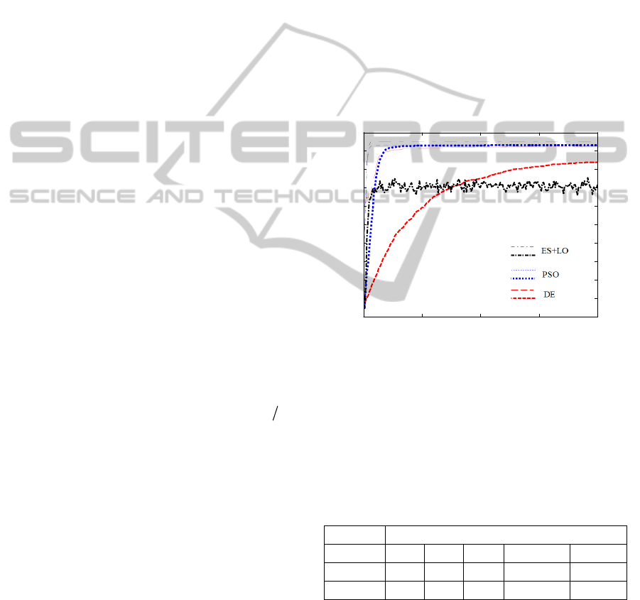
For the problem (9)-(10) sometimes are about to
stagnate, the average of the fitness function for every
population and the fitness of the best individual are
shown on the figure 3.
On the figure 3 there are next measurements:
dotted thin line is the best solution found by PSO at
the current iteration; dotted thick line is the average
fitness function value for the population; the same
with dashed lines for differential evolution and dot
dashed lines for ES. These lines are the averaging of
the presented variables after 20 restarts of algorithms
with the same settings. The horizontal axis is the
number of iteration for every algorithm; vertical axis
is the fitness function value. As one can see, the
PSO technique efficiency is more dependent on its
settings, because the whole population can fall to the
best solution found fast enough without possibility
to leave local extremum.
0 50 100 150 200
0
0.1
0.2
0.3
0.4
0.5
0.6
0.7
0.8
0.9
1
Figure 3: Behaviour of average fitness function value and
fitness of the best individual. Thick lines are the average
fitness and thin lines are the best fitness.
In table 1 the average values of the fitness function
for the found solution are presented. In every
column the efficiency with the best settings of every
technique are shown.
Table 1: Average values of the fitness function for
different techniques with the most efficient settings.
Algorithm
Problem ES DE PSO CMA-ES ES+LO
(7)-(8) 0.97 0.98 0.95 0.99 0.99
(9)-(10) 0.93 0.95 0.96 0.94 0.97
In table 2 the probability estimation of
1 ( *) 0.05
fitness op
is considered, since that is
the measurement of how the technique handle with
the complexity of objective function for the problem
(9)-(10).
AboutOptimizationTechniquesinApplicationtoSymbolic-NumericOptimalControlSeekingAproach
273
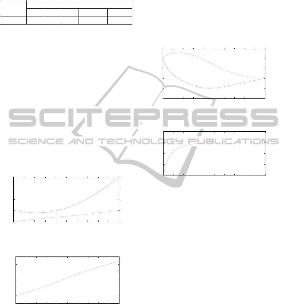
Table 2: The estimation of probability to return solution
that is close to the global optimum.
Algorithm
ES DE PSO CMA-ES ES+LO
Problem
0.3 0.5 0.6 0.35 0.65
In the current investigation, all the algorithms’
settings and population, individual numbers were
varied. Due to given problems, the hybrid
evolutionary strategies algorithm was the most
effective in searching the extremum and reliable in
case of the problems with objective function that
have a surface as it is shown on figure 2. After all
the runs, the best settings were estimated as
following ones: 20 individuals for 200 populations,
tournament selection (10%), discrete crossover,
modified mutation (mutation probability 0.75) and
12
/2
I
NNN ,
3
0.1N , with evaluations
number limitation equal to 8000.
For every of the proposed algorithms the most
efficient settings were estimated too. The balance
between the number of populations and size of
population differs from one method to another. For
example, PSO shows better results with increasing
the number of individuals, but DE does not.
0 0.1 0. 2 0.3 0.4 0.5 0.6 0.7 0.8 0.9 1
1
2
3
4
5
Figure 4: The system output for the control problem (7)-
(8),
12
(), ()
x
txt.
0 0. 1 0. 2 0. 3 0. 4 0. 5 0. 6 0. 7 0. 8 0. 9 1
-4
-2
0
2
4
6
8
Figure 5: Function ()ut . Control problem (7)-(8).
Let us consider the optimal control problem (7)-(8)
again. It has been shown earlier how we analytically
transformed the initial problem and closed the
system with state and co-state variables. The
modified hybrid evolutionary strategies algorithm
was applied for this control problem. After 20 runs
of the algorithm, the best solution was taken. The
state variables are shown on the Figure 4 and the
control function is shown on the Figure 5. As one
can see, system state with the given control reaches
the desired end point at time T.
For the problem (9)-(10), another 20 runs of the
ES+LO algorithm gave us solution that is shown on
the Figures 6 and 7.
0 0.5 1 1.5 2 2.5 3 3.5 4 4.5 5
-1
-0.5
0
0.5
1
1.5
Figure 6: The system output for the control problem (9)-
(10),
12
(), ()
x
txt.
0 0.5 1 1. 5 2 2.5 3 3.5 4 4.5 5
-6
-4
-2
0
2
Figure 7: Function ()ut . Control problem (9)-(10).
As it is shown in the given examples, the proposed
algorithm effectively solves the unconstrained
optimal control problem for nonlinear dynamic
systems. The initial point for co-state variables is to
be found, because after closing up the extended
system with state and co-state variables, regarding to
the maximum principle, the control function is fully
determined with them. As one can see, the proposed
approach does not guarantee that any optimal control
problem can be solved, but if the solution exists,
there is a chance for it to be found. Also, the
proposed approach fits only the optimal control
problems that can be analytically transformed and
the control function can be expressed via state and
co-state variables after closing the system.
The proposed approach is suitable for the
optimal control problems with different definitions,
only criterion for extremum problem on the real
vector field would be different.
5 CONCLUSIONS
In this study the analytically-numerical algorithm of
ICINCO2013-10thInternationalConferenceonInformaticsinControl,AutomationandRobotics
274

the optimal control problem solving for nonlinear
dynamic systems with one input and many outputs is
considered. The initial two-point optimal control
problem with integral functional was reduced to
extremum problem on real vectors field. With all the
transformations, listed above, the system with state
and co-state variables can be closed and the control
function structure can be defined in terms of the co-
state variables and system state. The seeking of
initial point for the co-state variables brings the
solution for the optimal control problem and
suggested to be based on stochastic or evolution
unconstrained global optimization algorithms.
As the optimization techniques evolutionary
strategies, differential evolution, particle swarm
optimization and their modifications were suggested
and investigated on the given optimal control
problems set. It is suggested that optimization
techniques with special features are required and
future works are related with designing hybrid
algorithms that allow both the extremum seeking
and surface scouting.
Since, there are plenty of different optimal
control problems, as the system equations and
functional differs from task to task, the mapping to
be optimized has different characteristics and there
is no set of the problems that allows making a
complete investigation of the optimization
algorithms efficiency. All in all, the investigation of
efficiency for heuristic techniques proceeds in the
same way, techniques are testing on the well-known
set of the objective functions. The proposed
approach leads to investigate the efficiency of
techniques with different extremum problem
definition, and it seems to be the only way to find
the most suitable algorithm by testing it on some set
of the control problems.
In the current investigation the hybrid
evolutionary strategies approach was the most
effective.
The aim of the further investigation is to design
the critique program agent, which will be the
controller for the optimization technique, via
analysing the data: fitness function set and its
history, the topology of the individuals and its
dynamics. The algorithms with implementation of
this agent probably will be more efficient for global
extremum problems.
REFERENCES
Popescu, M., Dumitrache, M., 2005: On the optimal
control of affine nonlinear systems. Mathematical
Problems in Engineering (4): pp. 465–475.
Chen, W. H., Balance, D. J., Gawthrop, P. J., 2003:
Optimal control of nonlinear systems: a predictive
control approach. Automatica 39(4): pp. 633-641.
Primbs, J. A., Nevistic, V., Doyle, J. C., 1999: Nonlinear
optimal control: a control Lyapunov function and
receding horizon perspective. Asian Journal of
Control, Vol. 1, No. 1: pp. 14-24.
Rao, A. V., 2009: Survey of Numerical methods for
Optimal Control, AAS/AIAA Astrodynamics
Specialist Conference, AAS Paper 09-334, Pittsburg,
PA.
Bertolazzi, E., Biral, F., Lio, M., 2005, Symbolic-Numeric
Indirect Method for Solving Optimal Control
Problems for Large Multibody Systems: The Time-
Optimal Racing Vehicle Example. Multibody System
Dynamics, Vol. 13, No. 2., pp. 233-252
Cruz, P., Torres, D., 2007, Evolution strategies in
optimization problems, Proc. Estonian Acad. Sci.
Phys. Math., 56, 4, pp. 299–309
Kirk, D. E., 1970: Optimal Control Theory: An
Introduction. Englewood Cliffs, NJ: Prentice-Hall.
Schwefel, H-P, 1995: Evolution and Optimum Seeking.
New York: Wiley & Sons.
Hansen, N., 2006: The CMA evolution strategy: a
comparing review. Towards a new evolutionary
computation. Advances on estimation of distribution
algorithms, Springer, pp. 1769–1776
Storn, R. Price, K.,1997: Differential Evolution - A Simple
and Efficient Heuristic for Global Optimization over
Continuous Spaces, Journal of Global Optimization,
11: pp. 341–359.
Kennedy, J., Eberhart, R., 2001: Swarm Intelligence.
Morgan Kaufmann Publishers, Inc., San Francisco,
CA.
AboutOptimizationTechniquesinApplicationtoSymbolic-NumericOptimalControlSeekingAproach
275
