
Singular and Non-singular Path Following Control
of a Wheeled Mobile Robot of (2,0) Type
Joanna Płaskonka
Institute of Computer Engineering, Control and Robotics, Wroclaw University of Technology,
Janiszewskiego 11/17, Wroclaw, Poland
Keywords:
Path Following, Wheeled Mobile Robot, Serret-Frenet Frame, Nonholonomic Constraints, Model-Based
Control.
Abstract:
This paper relates to the problem of a path following task for a wheeled mobile platform of (2,0) type. Two
kinematic control algorithms, Micaelli-Samson algorithm and Soetanto-Lapierre-Pascoal algorithm, which are
based on either the Serret-Frenet frame with an orthogonal projection or the Serret-Frenet frame with a non-
orthogonal projection of a robot on the desired path, were presented. The additional condition that should be
imposed on the function δ, which is a parameter depending on a linear velocity of the robot and on a distance
error, was described. The influence of the function δ on the convergence of the non-singular algorithm has
been shown using computer simulations.
1 INTRODUCTION
There are three groups of problems related to a motion
control of autonomous vehicles:
• point stabilization,
• trajectory tracking (the robot has to follow a de-
sired curve which is time-parametrized),
• path following (the task of the robot is to fol-
low a curve parametrized by a curvilinear distance
from a fixed point).
Various approaches to designing kinematic control
strategies for wheeled mobile robots can be used –
more general, which could be applied for few types
of mobile platforms, and dedicated to particular types
of wheeled mobile robots. Better results are usually
obtained for the latter ones. The examples of the al-
gorithms dedicated to a certain type of mobile robots
may be found e.g. in (Samson, 1992), (De Luca et al.,
1998), (Morro et al., 2011), (Płaskonka, 2012). One
can also consider a coordinated path following con-
trol for a group of wheeled mobile platforms, see e.g.
(Xiang et al., 2009), (Ronen and Arogeti, 2012).
Different ideas of describing the position of the
robot relative to the path were proposed in the litera-
ture. The one, which is the most commonly applied,
bases on the Serret-Frenet frame that moves along the
desired curve. In this paper two path parametrization
approaches are presented. In the first one the Serret-
Frenet frame is attached to the point on the path that
is closest to the robot, see e.g. (Samson, 1992), (Mi-
caelli and Samson, 1993). Unfortunately such an ap-
proach imposes on the vehicle stringent initial con-
ditions constraints. The second approach (Soetanto
et al., 2003) does not have such a drawback as the po-
sition of the virtual target to be tracked by the robot is
defined by a non-orthogonal projection of the vehicle
on the path. That approach inspired many scientists,
not only those who are focused on control algorithms
for mobile platforms, (Indiveri et al., 2007), (Xiang
et al., 2009), (Liu et al., 2012).
This paper addresses the problem of the realiza-
tion of a path following task by a wheeled mobile
robot of (2,0) type. The aim of the paper is to present
two path following algorithms, Micaelli-Samson al-
gorithm (Micaelli and Samson, 1993) and Soetanto-
Lapierre-Pascoal algorithm (Soetanto et al., 2003),
and indicate that one should take into account an ad-
ditional condition related to a function δ, that was
introduced in both of the mentioned kinematic con-
trol algorithms to broaden the control stability do-
main, which – to the best of author’s knowledge –
was not mentioned in the literature so far. In addition,
the influence of the function δ on the convergence of
Soetanto-Lapierre-Pascoal control algorithm has been
presented. The results of additional simulations pre-
senting the influence of values of controller’s param-
eters on the realization of the path following tasks
268
Plaskonka J..
Singular and Non-singular Path Following Control of a Wheeled Mobile Robot of (2,0) Type.
DOI: 10.5220/0004479202680275
In Proceedings of the 10th International Conference on Informatics in Control, Automation and Robotics (ICINCO-2013), pages 268-275
ISBN: 978-989-8565-71-6
Copyright
c
2013 SCITEPRESS (Science and Technology Publications, Lda.)
and simulations taking into account the velocity con-
straints have been provided as well.
2 MODEL OF A ROBOT
All wheeled mobile robots can be classified into one
of five generic types, (Campion et al., 1996). In this
paper the considerations will be restricted to a robot
belonging to the (2,0) type which is a two-wheel
differential-drive robot, also called in the literature
a unicycle. In general such a type of a robot con-
sists of a platform equipped with either one or several
fixed wheels with a common axle. It might also have
a passive caster wheel which serves as a support.
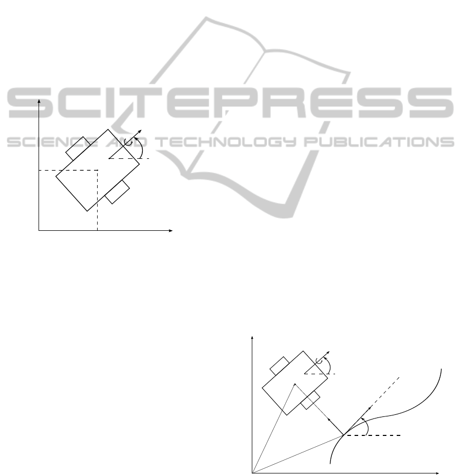
Fig. 1 depicts a unicycle which can be described
by generalized coordinates q = (x, y, θ)
T
. The point
θ
ω
v
M
X
0
Y
0
x
y
Figure 1: The unicycle’s parameters.
M (a robot’s guidance point) is located in the mid-
dle of the wheel axle of the vehicle. The variables
x and y denote the position of the point M relative
to the inertial frame, while θ is a robot’s orientation.
Taking into account the assumptions that the robot’s
wheels are non-deformable and the robot is moving
on a plane without slippage of its wheels, the kine-
matic model of the considered wheeled mobile robot
can be described by the equations
˙x = vcos θ,
˙y = vsin θ,
˙
θ = ω,
(1)
where symbols v and ω denote unicycle’s linear and
angular velocities, respectively.
3 DESCRIPTION OF THE ROBOT
RELATIVE TO A DESIRED
PATH
The position of the robot may be described not only
relative to an inertial frame, but also relative to a de-
sired path. For this purpose one may attach to a path
the Serret-Frenet frame which in general consists of
vectors tangent, normal and binormal to a desired
curve. The considered robot is moving on a plane so
in that case the Serret-Frenet frame consists only of
vectors tangent and normal to the path.
The main difference between a trajectory and a
path is that the first one is parametrized by the time,
while the latter one is parametrized by a curvilinear
distance s(t) from a fixed point, i.e. from the begin-
ning of the path. In other words, a trajectory is a spe-
cial case of a path when s(t) = t. The path P is char-
acterized by a curvature κ(s), which is the inversion
of the radius of the circle tangent to the path at a point
characterized by the parameter s. The desired orien-
tation of the mobile platform satisfies the equation
˙
θ
r
= ±κ(s) ˙s. (2)
The sign on the right side of the equation (2) de-
pends on the direction of moving along a desired
curve (negative when the Serret-Frenet frame moves
in the clockwise direction, positive otherwise).
3.1 The Serret-Frenet Frame with
an Orthogonal Projection
of a Robot on the Path
In this approach a virtual target to be tracked is de-
fined by the robot’s orthogonal projection on the de-
sired path, see Fig. 2. The point M’ is the orthogonal
X
0
Y
0
θ
ω
v
M
θ
r
P
p
1
q
1
r
1
M'
l
Figure 2: The Serret-Frenet frame definition in a case
of an orthogonal projection of a robot on the path.
projection of the point M on the path P and l is the
SingularandNon-singularPathFollowingControlofaWheeledMobileRobotof(2,0)Type
269

distance error between the actual vehicle and the vir-
tual one. The relationship between the position of the
point M relative to an inertial frame and its position
relative to the Serret-Frenet frame can be described
by the equation
q
1
1
=
R
θ
r
p
1
0 1
r
1
1
, (3)
where
R
θ
r
= R = Rot(z, θ
r
) =
cosθ
r
−sin θ
r
0
sinθ
r
cosθ
r
0
0 0 1
.
(4)
After differentiating and transforming the equation
(3), one has
˙
r
1
= R
T
˙
q
1
− R
T
˙
Rr
1
− R
T
˙
p
1
. (5)
Using the relationships
r
1
= (0 l 0)
T
, (6)
q
1
= (x y 0)
T
(7)
and
v
B
=
˙
R
T
˙
p
1
= ( ˙s 0 0)
T
, (8)
as the reference vehicle is moving along a desired path
in the direction of X axis of the Serret-Frenet frame,
the equation (5) can be rewritten as
0
˙
l
0
=
cosθ
r
sinθ
r
0
−sin θ
r
cosθ
r
0
0 0 1
˙x
˙y
0
+
−
0 −
˙
θ
r
0
˙
θ
r
0 0
0 0 0
0
l
0
−
˙s
0
0
, (9)
which leads to
˙
l = (−sinθ
r
cosθ
r
)
˙x
˙y
, (10)
˙s =
(cosθ
r
sinθ
r
)
1 ∓ κ(s)l
˙x
˙y
. (11)
To avoid singularity l = ±
1
κ(s)
one has to ensure that
during the control process an inequality |l κ(s)| < 1
holds, which means that the parametrization is local.
In addition, one can determine the orientation error
˜
θ = θ − θ
r
(12)
and its derivative
˙
˜
θ =
˙
θ −
˙
θ
r
=
˙
θ ∓ κ(s) ˙s. (13)
Finally the kinematic model of a wheeled mobile
robot of (2,0) type derived with respect to Serret-
Frenet frame can be described by the following sys-
tem of equations
˙
l = vsin
˜
θ,
˙s =
vcos
˜
θ
1∓κ(s)l
,
˙
˜
θ = ω ∓
κ(s)vcos
˜
θ
1∓κ(s)l
.
(14)
3.2 The Serret-Frenet Frame with
a Non-orthogonal Projection
of a Robot on the Path
The methodology described in this subsection avoids
the occurrence of the singularities which are present
in control strategies based on the approach presented
in subsection 3.1. This is done by using the Serret-
Frenet frame which is not attached to the point on the
path that is closest to the vehicle, see Fig. 3. As a re-
sult one has to take into account an extra controller
design parameter. In that situation there are three path
following errors – an orientation error
˜
θ and two dis-
tance errors, s
1
in the direction of the X axis and y
1
in the direction of Y axis of the Serret-Frenet frame.
Such an approach was proposed in (Soetanto et al.,
2003).
X
0
Y
0
θ
ω
v
M
θ
r
P
p
2
q
2
r
2
M'
s
1
y
1
Figure 3: The Serret-Frenet frame definition in a case
of a non-orthogonal projection of a robot on the path.
The velocity of r
2
is equal to
˙
r
2
= R
T
˙
q
2
− R
T
˙
Rr
2
− R
T
˙
p
2
(15)
with
r
2
= (s
1
y
1
0)
T
, (16)
q
2
= (x y 0)
T
(17)
and
˙
R
T
˙
p
2
= ( ˙s 0 0)
T
. (18)
From (15) one gets
˙s
1
˙y
1
0
=
cosθ
r
sinθ
r
0
−sin θ
r
cosθ
r
0
0 0 1
˙x
˙y
0
+
−
0 −
˙
θ
r
0
˙
θ
r
0 0
0 0 0
s
1
y
1
0
−
˙s
0
0
(19)
ICINCO2013-10thInternationalConferenceonInformaticsinControl,AutomationandRobotics
270

and thus
˙s
1
=
cosθ
r
sinθ
r
˙x
˙y
− ˙s(1 − y
1
κ(s)), (20)
˙y
1
=
−sin θ
r
cosθ
r
˙x
˙y
− ˙sκ(s)s
1
. (21)
There is no singularity related to distance errors in
equations (20)-(21). For the unicycle the kinematic
model expressed with respect to the Serret-Frenet
frame with a non-orthogonal projection of a robot
on the path is given by the following equations
˙s
1
= − ˙s(1 − κ(s)y
1
) + vcos
˜
θ,
˙y
1
= −κ(s) ˙ss
1
+ vsin
˜
θ,
˙
˜
θ = ω ∓κ(s) ˙s.
(22)
4 PATH FOLLOWING
ALGORITHMS
The considered control problem is to design a kine-
matic control law such that the wheeled mobile robot
of (2,0) type follows a desired path and path follow-
ing errors converge to zero. The desired path has to
be admissible, i.e. it can be realized without slippage
of robot’s wheels.
It is assumed that a direction of a movement along
the desired curve is opposite to the clockwise direc-
tion, this means that
˙
˜
θ = κ(s) ˙s. (23)
Hence the equations describing path following er-
rors for a case of an orthogonal projection of a robot
on the path have a form as below
˙
l = vsin
˜
θ,
˙
˜
θ = ω −
κ(s)vcos
˜
θ
1−κ(s)l
.
(24)
and in a case of a non-orthogonal projection are equal
to
˙s
1
= − ˙s(1 − κ(s)y
1
) + vcos
˜
θ,
˙y
1
= −κ(s) ˙ss
1
+ vsin
˜
θ,
˙
˜
θ = ω −κ(s) ˙s.
(25)
4.1 Singular Control Algorithm
Micaelli-Samson kinematic control law (Micaelli and
Samson, 1993) for the system (24) is equal to
ω =
κ(s)vcos
˜
θ
1−κ(s)l
+
∂δ(l,v)
∂l
vsin
˜
θ +
∂δ(l,v)
∂v
˙v +
− λ
˜
θ
h
f
∂ f
∂l
v
sin
˜
θ−sinδ(l,v)
˜
θ−δ(l,v)
− k|v|(
˜
θ − δ(l, v))
i
,
k > 0, λ
˜
θ
> 0,
(26)
where v(t) and ˙v(t) are bounded, v(t) does not tend to
zero when t tends to infinity, the functions
f (l) : (−r, r) → R
and
δ(l, v) : R × R → R
are C
2
and C
1
respectively and the following condi-
tions are satisfied:
• f (±r) = ±∞,
• f (0) = δ(0, v) = 0,
•
∂ f
∂l
(l) > 0, ∀l,
• v f (l)sin δ(l, v) ≤ 0,∀l, ∀v.
The function δ was introduced to set the desired val-
ues for the orientation error
˜
θ during transients. What
is more, the following inequality should hold
|δ(l, v)| <
π
2
, ∀l, ∀v. (27)
The system (24) with a closed-loop of the feedback
signal (26) is asymptotically stable. In addition, if
f (l) tends to infinity when l tends to
1
κ
max
, it is pos-
sible to keep l(t) in the open interval
−
1
κ
max
,
1
κ
max
when l(0) belongs to this interval.
Proof. Consider the Lyapunov function
V
1
=
1
2
f
2
(l) +
1
λ
˜
θ
˜
θ − δ(l, v)
2
. (28)
The time-derivative of V
1
˙
V
1
= f
∂ f
∂l
˙
l +
1
λ
˜
θ
(
˜
θ − δ)(
˙
˜
θ −
˙
δ) =
= f
∂ f
∂l
vsin δ + (
˜
θ − δ)[
1
λ
˜
θ
(ω+
−
κ(s)vcos
˜
θ
1−κ(s)l
−
∂δ
∂l
vsin
˜
θ −
∂δ
∂v
˙v)+
+ f
∂ f
∂l
v
sin
˜
θ−sinδ
˜
θ−δ
] =
= f
∂ f
∂l
vsin δ − k|v|(
˜
θ − δ)
2
(29)
is non-positive. This means that lim
t→∞
V
1
(t) = V
1lim
and f (l) and (
˜
θ − δ) are bounded.
˙
V
1
is uniformly
continuous because its derivative is bounded as sum
of bounded functions. By Barbalat’s lemma
˙
V
1
tends
to zero. Therefore f
∂ f
∂l
vsin δ → 0 and v(
˜
θ − δ) → 0.
Differentiating (
˜
θ − δ) with respect to time gives
d
dt
˜
θ − δ
= −λ
˜
θ
f
∂ f
∂l
v
sin
˜
θ−sinδ
˜
θ−δ
+
−k λ
˜
θ
|v|(
˜
θ − δ).
(30)
Hence
d
dt
[v
2
˜
θ − δ
] = 2v ˙v(
˜
θ − δ) − λ
˜
θ
f
∂ f
∂l
v
3
sin
˜
θ−sinδ
˜
θ−δ
+
−k λ
˜
θ
|v|v
2
(
˜
θ − δ)
(31)
SingularandNon-singularPathFollowingControlofaWheeledMobileRobotof(2,0)Type
271

is the sum of two terms which tend to zero and third
term which is uniformly continuous. As v
2
(
˜
θ − δ)
tends to zero, the extension of Barbalat’s lemma (Mi-
caelli and Samson, 1993) tells us that
d
dt
[v
2
˜
θ − δ
]
also tends to zero which implies that the term
λ
˜
θ
f
∂ f
∂l
v
3
sin
˜
θ−sinδ
˜
θ−δ
→ 0. The expression
sin
˜
θ−sinδ
˜
θ−δ
re-
quires a special comment. It can be rewritten in the
following way
sin
˜
θ − sinδ
˜
θ − δ
=
sin
˜
θ−δ
2
cos
˜
θ+δ
2
˜
θ−δ
2
(32)
which for (
˜
θ − δ) → 0 tends to cos δ or one can also
notice that for (
˜
θ − δ) → 0 the expression
sin
˜
θ−sinδ
˜
θ−δ
is
equal to the derivative of the sine function. If only
δ does not tend to
mπ
2
, m ∈ Z, the the whole term
sin
˜
θ−sinδ
˜
θ−δ
does not tend to zero. This fact was not
indicated in (Micaelli and Samson, 1993). It seems
reasonable to assume that δ should be less than
π
2
for all l and for all v. Under this assumption f
∂ f
∂l
v
tends to zero. At the beginning it was assumed that
∂ f
∂l
(l) > 0 which leads to v f → 0. Using the facts that
v(
˜
θ−δ) → 0 and v f → 0, one may conclude that v
2
V
1
tends to zero and V
1lim
= 0. Thus both f and (
˜
θ − δ)
tend to zero. From the properties of the function f , l
also tends to zero and therefore δ → 0. Finally one
conclude that
˜
θ tends to zero which completes the
proof.
4.2 Non-singular Control Algorithm
The control algorithm proposed in (Soetanto et al.,
2003) for the system (25) is equal to
˙s = v cos
˜
θ + k
1
s
1
,
ω = κ(s) ˙s +
˙
δ(y
1
, v) − γy
1
v
sin
˜
θ−sinδ(y
1
,v)
˜
θ−δ(y
1
,v)
+
− k
2
(
˜
θ − δ(y
1
, v)),
k
1
, k
2
> 0, γ = const,
(33)
where the following assumptions have been made
• lim
t→∞
v(t) 6= 0, e.g. v = const,
• δ(0, v) = 0,
• ∀
y
1
∀
v
y
1
vsin δ(y
1
, v) ≤ 0.
What is more, the following inequality should hold
|δ(y
1
, v)| <
π
2
, ∀y
1
, ∀v, (34)
which was not mentioned in (Soetanto et al., 2003).
The control algorithm guarantees the convergence of
y
1
, s
1
and
˜
θ to zero. That can be shown using the
following Lyapunov function
V
2
=
1
2
(s
2
1
+ y
2
1
) +
1
2γ
(
˜
θ − δ(y
1
, v))
2
(35)
and carrying out the similar reasoning to one which
was presented in the subsection 4.1. The complete
proof of the convergence can be found in (Płaskonka,
2013).
5 SIMULATION RESULTS
The simulations were carried out to illustrate the be-
haviour of the wheeled mobile robot of (2,0) type
with the non-singular Soetanto-Lapierre-Pascoal con-
troller. The initial position of the platform was equal
to (x
0
, y
0
, θ
0
) = (12, 2,
π
4
). The desired path was the
circle described by the equations
x(s) = R cos
s
R
,
y(s) = Rsin
s
R
,
where R = 2 m.
5.1 The Influence of Different Values
of δ Function on the Realization
of the Task
Parameters of the kinematic controller were set to the
values presented below:
• v = 1,
• k
1
= 1,
• k
2
= 1000,
• γ = 1,
• θ
a
= {
π
4
,
π
2
, π, 2π},
• δ = −sign(v)θ
a
tanhy
1
.
The results of the simulations were presented in
Fig. 4-11.
Figure 4: The path following for the unicycle, XY plot
(Soetanto-Lapierre-Pascoal algorithm, θ
a
=
π
4
).
ICINCO2013-10thInternationalConferenceonInformaticsinControl,AutomationandRobotics
272
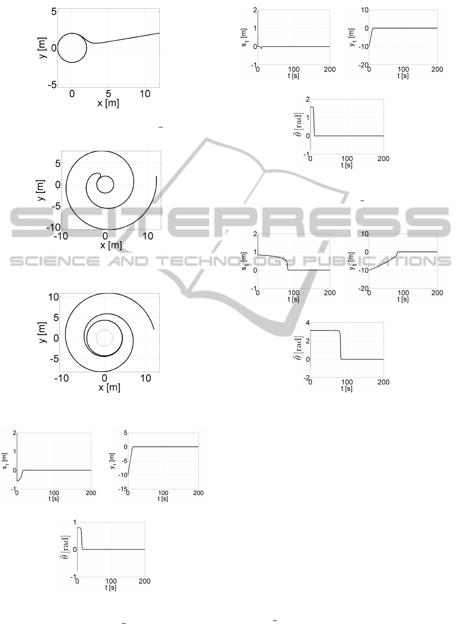
Figure 5: The path following for the unicycle, XY plot
(Soetanto-Lapierre-Pascoal algorithm, θ
a
=
π
2
).
Figure 6: The path following for the unicycle, XY plot
(Soetanto-Lapierre-Pascoal algorithm, θ
a
= π).
Figure 7: The path following for the unicycle, XY plot
(Soetanto-Lapierre-Pascoal algorithm, θ
a
= 2π).
(a) (b)
(c)
Figure 8: The path following for the unicycle (Soetanto-
Lapierre-Pascoal algorithm, θ
a
=
π
4
): (a) the distance error
s
1
, (b) the distance error y
1
, (c) the orientation error
˜
θ.
(a) (b)
(c)
Figure 9: The path following for the unicycle (Soetanto-
Lapierre-Pascoal algorithm, θ
a
=
π
2
): (a) the distance error
s
1
, (b) the distance error y
1
, (c) the orientation error
˜
θ.
(a) (b)
(c)
Figure 10: The path following for the unicycle (Soetanto-
Lapierre-Pascoal algorithm, θ
a
= π): (a) the distance error
s
1
, (b) the distance error y
1
, (c) the orientation error
˜
θ.
5.2 The Influence of Different Values
of k
i
Parameters on the Realization
of the Task
Parameters of the kinematic controller were set to the
values presented below:
• v = 1,
• k
1
= {0.1, 1, 10, 100, 1000, 10000},
• k
2
= {0.1, 1, 10, 100, 1000, 10000},
• γ = 1,
• θ
a
=
π
4
,
• δ = −sign(v)θ
a
tanhy
1
.
SingularandNon-singularPathFollowingControlofaWheeledMobileRobotof(2,0)Type
273
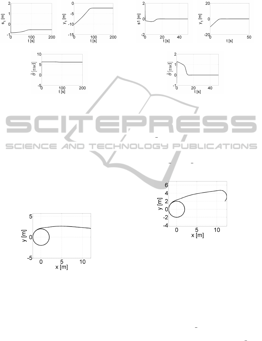
(a) (b)
(c)
Figure 11: The path following for the unicycle (Soetanto-
Lapierre-Pascoal algorithm, θ
a
= 2π): (a) the distance error
s
1
, (b) the distance error y
1
, (c) the orientation error
˜
θ.
The chosen quality indicator for the presented algo-
rithm is equal to
Q =
3
∑
k=1
I
k
+
2
∑
j=1
Z
T
0
u
2
j
,
where I
1
=
R
T
0
s
2
1
dt, I
2
=
R
T
0
y
2
1
dt, I
3
=
R
T
0
˜
θ
2
dt and
u
1
, u
2
are control inputs. Table 1 presents values of Q
for selected values of the control parameters k
i
. The
quality indicator reached the minimum for k
1
= 1 and
k
2
= 10. The results of the simulations for those pa-
rameters were presented in Fig. 12-13.
Figure 12: The path following for the unicycle, XY plot
(Soetanto-Lapierre-Pascoal algorithm, k
1
= 1, k
2
= 10).
5.3 The Simulations Taking into
Account Velocity Constraints
Parameters of the kinematic controller were set to the
values presented below:
• v = 1,
• k
1
= 1,
• k
2
= 10,
• γ = 1,
(a) (b)
(c)
Figure 13: The path following for the unicycle (Soetanto-
Lapierre-Pascoal algorithm, k
1
= 1, k
2
= 10): (a) the dis-
tance error s
1
, (b) the distance error y
1
, (c) the orientation
error
˜
θ.
• θ
a
=
π
4
,
• δ = −sign(v)θ
a
tanhy
1
.
The velocity constraint imposed on the on the robot
is chosen as −
π
5
≤ ω ≤
π
5
[rad/s]. The results of the
simulations were presented in Fig. 14-15.
Figure 14: The path following for the unicycle, XY plot
(Soetanto-Lapierre-Pascoal algorithm, simulations taking
into account velocity constraints).
6 CONCLUSIONS
In the paper singular and non-singular kinematic path
following controllers have been presented. It was sug-
gested to take into account an additional condition im-
posed on the function δ which is a parameter of both
algorithms. According to that condition the values of
δ should be smaller than
π
2
. The simulations of the
Soetanto-Lapierre-Pascoal algorithm have shown that
it is reasonable to limit values of δ. For θ
a
>
π
2
the
convergence of the algorithm was unacceptably slow.
Simulation analysis has shown that the presented al-
gorithm works properly for different values of the k
i
ICINCO2013-10thInternationalConferenceonInformaticsinControl,AutomationandRobotics
274
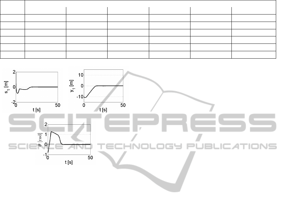
Table 1: The values of the quality indicator Q obtained in the simulations for selected values of k
i
parameters.
k
1
k
2
0.1 1 10 100 1000 10 000
0.1 631.9 513.2 512.4 681.9 1 801.3 12 835.6
1 607.3 514.2 490.1 664.3 1 789.1 12 824.1
10 626.3 518.7 497.5 699.0 1 836.5 12 873.4
100 635.9 526.5 506.1 734.4 2 013.2 13 148.5
1000 710.4 600.8 580.5 815.6 2 339.1 14 886.6
10 000 1 438.4 1 328.3 1 307.9 1 543.8 3 131.6 18 164.1
(a) (b)
(c)
Figure 15: The path following for the unicycle (Soetanto-
Lapierre-Pascoal algorithm, simulations taking into account
velocity constraints): (a) the distance error s
1
, (b) the dis-
tance error y
1
, (c) the orientation error
˜
θ.
parameters, however choosing large values of the con-
troller’s parameters is undesirable due to a significant
control cost. What is more, the path following task is
realized correctly by the considered wheeled mobile
robot when the Soetanto-Lapierre-Pascoal algorithm
is modified by adding velocity constraints.
An extension of this work could be testing if the
other kinds of δ function, not necessarily sigmoid-
like, could be applied for the presented algorithms.
REFERENCES
Campion, G., Bastin, G., and d’Andr
´
ea Novel, B. (1996).
Structural properties and classification of kinematic
and dynamic models of wheeled mobile robots. IEEE
Transactions on Robotics and Automation, 12(5):47–
61.
De Luca, A., Oriolo, G., and Samson, C. (1998). Feed-
back control of a nonholonomic car-like robot. In
Laumond, J.-P., editor, Robot Motion Planning and
Control, pages 171–253. Springer-Verlag.
Indiveri, G., Nuchter, A., and Lingemann, K. (2007). High
speed differential drive mobile robot path following
control with bounded wheel speed commands. Pro-
ceedings of the 2007 IEEE International Conference
on Robotics and Automation, pages 2202–2207.
Liu, C., McAree, O., and Chen, W.-H. (2012). Path fol-
lowing for small UAVs in the presence of wind dis-
turbance. Proceedings of the UKACC International
Conference on Control, pages 613–618.
Micaelli, A. and Samson, C. (1993). Trajectory tracking for
unicycle-type and two-steering-wheels mobile robots.
Technical Report No. 2097, INRIA, Sophia-Antipolis,
France.
Morro, A., Sgorbissa, A., and Zaccaria, R. (2011). Path fol-
lowing for unicycle robots with an arbitrary path cur-
vature. IEEE Transactions on Robotics, 27(5):1016–
1023.
Płaskonka, J. (2012). The path following control of a uni-
cycle based on the chained form of a kinematic model
derived with respect to the Serret-Frenet frame. Pro-
ceedings of 17th International Conference on Methods
and Models in Automation & Robotics, MMAR 2012,
27(5):1016–1023.
Płaskonka, J. (2013). Different kinematic path following
controllers for a wheeled mobile robot of (2,0) type.
Sent for publication.
Ronen, R. and Arogeti, S. (2012). Coordinated path follow-
ing control for a group of car-like vehicles. Proceed-
ings of the IEEE 12th International Conference on
Control, Automation, Robotics & Vision, pages 719–
724.
Samson, C. (1992). Path following and time-varying feed-
back stabilization of a wheeled mobile robots. Pro-
ceedings of the IEEE Int. Conf. on Advanced Robotics
and Computer Vision, pages 1.1–1.5.
Soetanto, D., Lapierre, L., and Pascoal, A. (2003). Adap-
tive, non-singular path-following control of dynamic
wheeled robots. Proceedings of the IEEE Conference
on Decision and Control, 2:1765–1770.
Xiang, X., Lapierre, L., Jouvencel, B., and Parodi, O.
(2009). Coordinated path following control of mul-
tiple wheeled mobile robots through decentralized
speed adaptation. Proceedings of the IEEE/RSJ In-
ternational Conference on Intelligent Robots and Sys-
tems, pages 4547–4552.
SingularandNon-singularPathFollowingControlofaWheeledMobileRobotof(2,0)Type
275
