
Stabilization of a Trajectory for Nonlinear Systems using the
Time-varying Pole Placement Technique
Yasuhiko Mutoh and Shuhei Naitoh
Department of Engineering and Applied Sciences, Sophia University, 7-1, Kioicho, Chiyoda-ku, Tokyo, Japan
Keywords:
Stabilization of Trajectory, Nonlinear System, Linear Time-varying System, Pole Placement.
Abstract:
The author proposed the simple design procedure of pole placement controller for linear time-varying systems.
The feedback gain can be obtained directly from the plant parameters without transforming the system into any
standard form. This design method will be applied to the problem of stabilization of some desired trajectory
of nonlinear systems.
1 INTRODUCTION
In general, to design a controller for nonlinear sys-
tems, we approximate the system around some equi-
librium point by a linear time-invariant system, and
then, linear control design methods are applied. But,
if we need to stabilize some particular trajectory, in
practice, we approximate the nonlinear system around
multiple points for designing the controller. In such a
case, gain scheduling method or some other similar
scheme will be necessary. Nonlinear controllers, of
course, are one of other choices. The most simple idea
is to approximate the nonlinear system around some
trajectory using a linear time-varying system. How-
ever, since, the design method for linear time-varying
systems is not necessarily simple (Nguyen(1987))
(Valsek(1995)) (Valsek(1999)), the gain scheduling
strategy may be the first choice for such a control de-
sign problem, in general. The author et. al. have
proposed simple pole placement controller design
method (Mutoh(2011))(Mutoh and Kimura (2011)).
Such controller is obtained by finding a new output
signal so that the relative degree from the input to this
new output is equal to the system degree. We do not
need to transform the system into any standard form
for the controller design. In this paper, such a pole
placement controller design procedure will be applied
to the problem of the stabilization of some desired tra-
jectory of nonlinear systems. Section 2 will present
how to design the pole placement controller for lin-
ear time-varying systems. For the simplicity, we con-
sider only single-input single-output systems. Then,
Section 3 will show an example of stabilizing some
desired trajectory of a nonlinear system.
2 POLE PLACEMENT FOR
LINEAR TIME-VARYING
SYSTEMS
Consider the following linear time-varying system.
˙x = A(t)x+ b(t)u (1)
Here, x(t) ∈ R
n
is the state vector and u(t) ∈ R
1
is the
input signal. A(t) ∈ R
n×n
and b(t) ∈ R
n
are time vary-
ing coefficient matrices, which are smooth functions
of t.
The controllability matrix, U
c
(t), of this system is
U
c
(t) = [b
0
(t), b
1
(t), ··· , b
n−1
(t)] (2)
where b
i
(t) is defined by the following recurrence
equation.
b
0
(t) = b(t)
b
i
(t) = A(t)b
i−1
(t) −
˙
b
i−1
(t), i = 1, 2, ···
(3)
The system (1) is controllable if and only if U
c
(t) is
nonsingular for all t.
The problem is to find the state feedback
u(t) = k
T
(t)x(t) (4)
for the system (1) which makes the closed loop sys-
tem equivalent to some time invariant linear system
with arbitrarily stable poles.
For this purpose, consider the problem of finding a
new output signal y such that the relative degree from
u to y is n. Here, y has the following form.
y = c
T
(t)x (5)
410
Mutoh Y. and Naitoh S..
Stabilization of a Trajectory for Nonlinear Systems using the Time-varying Pole Placement Technique.
DOI: 10.5220/0004478804100416
In Proceedings of the 10th International Conference on Informatics in Control, Automation and Robotics (ICINCO-2013), pages 410-416
ISBN: 978-989-8565-70-9
Copyright
c
2013 SCITEPRESS (Science and Technology Publications, Lda.)

Then, the problem is to find a vector c(t) ∈ R
n
that
satisfies this condition.
Let c
T
i
(t) be defined by
c
T
0
(t) = c
T
(t)
c
T
i
(t) = ˙c
T
i−1
(t) + c
T
i−1
(t)A(t), i = 1, 2, ···
(6)
Then, we have the following lemma.
Lemma 1. The relative degree from u to y is n if and
only if
c
T
0
(t)b(t) = 0
c
T
1
(t)b(t) = 0
.
.
.
c
T
n−2
(t)b(t) = 0
c
T
n−1
(t)b(t) = λ(t), λ(t) 6= 0
(7)
Proof: By differentiating y successively, we have the
following equations from (7).
y = c
T
(t)x
= c
T
0
(t)x
˙y =
˙c
0
T
(t) + c
T
0
(t)A(t)
x+ c
T
0
(t)b(t)u
= c
T
1
(t)x+ c
T
0
(t)b(t)u
= c
T
1
(t)x
¨y =
˙c
T
1
(t) + c
T
1
(t)A(t)
x+ c
T
1
(t)b(t)u
= c
T
2
(t)x+ c
T
1
(t)b(t)u
= c
T
2
(t)x
.
.
.
y
(n−1)
= c
T
n−1
(t)x+ c
T
n−2
(t)b(t)u
= c
T
n−1
(t)x
y
(n)
= c
T
n
(t)x+ c
T
n−1
(t)b(t)u
= c
T
n
(t)x+ λ(t)u
(8)
This implies that the relative degree from u to y be-
comes n and vice versa. Note that λ(t) = 1 can be a
simple choice. But, as shown later in examples, some
particular choice for λ(t) makes a design calculation
simpler.
Lemma 2. If the relative degree from u to y = c
T
(t)x
is n, we have the following relation.
[c
T
0
(t)b(t), c
T
1
(t)b(t), · ·· , c
T
n−1
(t)b(t)]
= [c
T
(t)b
0
(t), c
T
(t)b
1
(t), · ·· , c
T
(t)b
n−1
(t)]
(9)
Proof: From (3) and (6),
c
T
0
(t)b(t) = c
T
(t)b(t) = c
T
(t)b
0
(t) (10)
Using (7), we have
˙c
T
0
(t)b(t) = −c
T
0
(t)
˙
b(t) (11)
and then,
c
T
1
(t)b(t) = ˙c
T
0
(t)b(t) + c
T
0
(t)A(t)b(t)
= −c
T
0
(t)
˙
b(t) + c
T
0
(t)A(t)b(t)
= c
T
0
(t)b
1
(t)
= c
T
(t)b
1
(t) (12)
Similarly, using (7), the following relations are ob-
tained.
˙c
T
0
(t)b
1
(t) = −c
T
0
(t)
˙
b
1
(t)
˙c
T
1
(t)b(t) = −c
T
1
(t)
˙
b(t)
(13)
From which we have
c
T
2
(t)b(t) = ˙c
T
1
(t)b(t) + c
T
1
(t)A(t)b(t)
= −c
T
1
(t)
˙
b(t) + c
T
1
(t)A(t)b(t)
= c
T
1
(t)b
1
(t)
= ˙c
T
0
(t)b
1
(t) + c
T
0
(t)A(t)b
1
(t)
= −c
T
0
(t)
˙
b
1
(t) + c
T
0
(t)A(t)b
1
(t)
= c
T
0
(t)b
2
(t)
= c
T
(t)b
2
(t) (14)
By continuing this operation, (9) is obtained.
From the above, (9) can be written as
[c
T
0
(t)b(t),c
T
1
(t)b(t),··· , c
T
n−1
(t)b(t)]
= c
T
(t)U
c
(t)
= [0, 0, ··· , λ(t)] (15)
then, we have the following Theorem.
Theorem 1. If the system (1) is controllable, a time
varying vector, c
T
(t), such that the relative degree
from u to a new output y = c
T
(t)x is n, can be ob-
tained by the following equation.
c
T
(t) = [0, 0, ··· , λ(t)]U
−1
c
(t) (16)
Let the stable characteristic polynomial of the desired
linear time invariant system be
q(p) = p
n
+ α
n−1
p
n−1
+ ··· + α
0
(17)
where p is a differential operator. By multiplying i-th
equation of (8) α
i
(α
n
= 1) and summing them up, we
have
q(p)y = d
T
(t)x+ λ(t)u (18)
where d
T
(t) is defined by
d
T
(t) = [α
0
,α
1
,··· , α
n−1
,1]
c
T
0
(t)
c
T
1
(t)
.
.
.
c
T
n−1
(t)
c
T
n
(t)
(19)
Then, by the state feedback
u = −
1
λ(t)
d
T
(t)x (20)
StabilizationofaTrajectoryforNonlinearSystemsusingtheTime-varyingPolePlacementTechnique
411

a new output y satisfies the following closed loop sys-
tem equation.
q(p)y = 0 (21)
This implies that by applying the state feedback (20)
to the system (1), the closed loop state equation be-
comes
˙x = (A(t) − b(t)d
T
(t))x. (22)
Then, from (8), using the state transformation matrix
T(t) =
c
T
0
(t)
c
T
1
(t)
.
.
.
c
T
n−1
(t)
(23)
the following state transformation can be defined.
ξ = T(t)x (24)
where
ξ =
y(t)
˙y(t)
.
.
.
y
(n−1)
(t)
(25)
Then, (21) implies that the closed loop system (22) is
equivalent to some linear time-invariant system that
has desired stable eigenvalues, i.e.,
˙
ξ = {T(t)(A(t) − b(t)d
T
(t))T
−1
(t) − T (t)
˙
T
−1
(t)}ξ
=
0 1 ··· 0
.
.
.
.
.
.
.
.
.
.
.
. 1
−α
0
··· ·· · −α
n−1
ξ
= A
∗
ξ
(26)
where, the characteristic polynomial of A
∗
is q(s) in
(17).
As for the nonsingularity of T(t), we have the fol-
lowing Theorem.
Theorem 2. If the system (1) is controllable, T(t) de-
fined by (23) is nonsingular.
Proof: From (3) and (6),
c
T
k+1
(t)b
j
(t) = ˙c
T
k
(t)b
j
(t) + c
T
k
(t)A(t)b
j
(t)
= −c
T
k
(t)
˙
b
j
(t) + c
T
k
(t)A(t)b
j
(t)
= c
T
k
(t)b
j+1
(t) (27)
Then, from (7),
c
T
0
(t)b
0
(t) = 0
.
.
.
c
T
0
(t)b
n−2
(t) = 0
c
T
0
(t)b
n−1
(t) = λ(t)
(28)
hence,
T(t)U
c
(t) =
c
T
0
(t)
.
.
.
c
T
n−1
(t)
b
0
(t) ··· b
n−1
(t)
=
0 ··· λ(t)
.
.
.
.
.
.
.
.
.
λ(t) · ·· ∗
(29)
which implies that if the system (1) is controllable,
T(t) is nonsingular.
The transformation matrix T(t) of a linear time-
varying system is called a Lyapunov transformation if
both of T(t) and T
−1
(t) are continuous and bounded
function of t (Chen(1999)). It is known that if T(t)
is a Lyapunov transformation matrix, ˙x = A(t)x is
uniformly exponentially stable if and only if ˙x =
{T(t)A(t)T
−1
(t) − T(t)
˙
T
−1
(t)}x is uniformly expo-
nentially stable (Rugh(1987)). Hence, T(t) should be
a Lyapunov transformation matrix for the pole place-
ment closed loop system to be uniformly exponen-
tially stable.
In summary, when the linear time-varying system
(1) is given, the design procedure of the pole place-
ment is as follows.
[Pole Placement Design Procedure].
[STEP 1]. Calculate U
c
(t) according to (2) and (3),
and check the controllability of the system.
[STEP 2]. Calculate c
T
(t) using (16).
[STEP 3]. Calculate c
T
0
(t), c
T
1
(t), ···, c
T
n−1
(t) from
A(t) and c
T
(t) using (6).
[STEP 4]. Determine the desired stable characteris-
tic polynomial q(s) in (17) and d
T
(t) by (19). Then
the pole placement state feedback is obtained as u =
−
1
λ(t)
d
T
(t)x.
3 STABILIZATION OF
A TRAJECTORY FOR
NONLINEAR SYSTEMS
In this section, we consider the stabilization prob-
lem of some particular trajectory of a nonlinear sys-
tem. For this purpose, we approximate the nonlinear
system by using a linear time-varying system around
some desired trajectory. And then, the simplified pole
placement controller design procedure will be applied
to stabilize this trajectory.
Consider the following nonlinear system.
˙x(t) = f(x(t),u(t)) (30)
ICINCO2013-10thInternationalConferenceonInformaticsinControl,AutomationandRobotics
412
Here, x(t) ∈ R
n
and u(t) ∈ R
1
are the state vector and
the input signal. Let x
∗
(t) and u
∗
(t) be some desired
trajectory and desired input signal, that is,
˙x
∗
(t) = f(x
∗
(t), u
∗
(t)), x
∗
(0) = x
∗
0
(31)
where the initial state, x
∗
0
is on the desired trajectory.
Let ∆x(t) and ∆u(t) be defined by
∆x(t) = x(t) − x
∗
(t)
∆u(t) = u(t) − u
∗
(t) (32)
Then, (30) can be approximated by the following lin-
ear time-varying system arround around (x
∗
(t), u
∗
(t)).
∆˙x(t) = A(t) ˙x(t) + b(t)∆u(t) (33)
where
A(t) =
∂
∂x
f(x
∗
(t), u
∗
(t))
b(t) =
∂
∂u
f(x
∗
(t), u
∗
(t)) (34)
Here, A(t) and b(t) may be known as their explicit
form of functions or known as numerical data. In any
case, the pole placement controller design procedure
can be applied to stabilize ∆x(t).
[EXAMPLE 1].
Consider the following Van Der Pol equation as
an example of a nonlinear system.
¨y+ (1− y
2
) ˙y+ y = 0 (35)
This equation can be presented by the following state
equation.
(
˙x
1
= x
2
˙x
2
= −x
1
− (1− x
2
1
)x
2
+ f(u)
(36)
Here, we put u as a control input, and it is supposed
that u affects the system through the nonlinear func-
tion
f(u) = 2(
2
1+ exp(−0.5u)
− 1). (37)
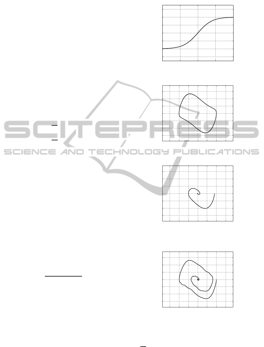
This function is shown in Fig.1.
This system has an unstable limit cycle shown in
Fig.2 when the u(t) = 0. In fact, the trajectory moves
away from the limit cycle as shown in Fig.3 if the
inieial condition is slightly away from the limit cicle
(x
1
(0) = 1.8, x
2
(0) = 0). As well, Fig.4 shows the
trajectory when a disturbance 0.5sin(10t) is added to
the input signal with its initial condition on the limit
cicle.
The linear time-varying system that approximate
this nonlinear system around the unstable limit cycle
x
∗
1
(t), x
∗
2
(t) is written as follows.
−10 −5 0 5 10
−3
−2
−1
0
1
2
3
u(t)
f(u)
Figure 1: Nonlinear Input Function.
−3 −2 −1 0 1 2 3
−3
−2
−1
0
1
2
3
X1
X2
Figure 2: Limit Cycle of the System.
−3 −2 −1 0 1 2 3
−3
−2
−1
0
1
2
3
X1
X2
Figure 3: State Response with the Initial Condition near the
Limit Cycle.
−3 −2 −1 0 1 2 3
−3
−2
−1
0
1
2
3
X1
X2
Figure 4: Disturbed State Response with the Initial Condi-
tion on the Limit Cycle.
d
dt
∆x
1
(t)
∆x
2
(t)
= A(t)
∆x
1
(t)
∆x
2
(t)
+ b(t)∆u
(38)
where ∆x
1
(t) = x
1
(t) − x
∗
1
(t), ∆x
2
(t) = x
2
(t) − x
∗
2
(t),
StabilizationofaTrajectoryforNonlinearSystemsusingtheTime-varyingPolePlacementTechnique
413
∆u(t) = u(t) − 0, and, from (34), A(t) and b(t) are
defined by the following equations.
A(t) =
0 1
−1+ 2x
∗
1
(t)x
∗
2
(t) −1+ x
∗2
1
(t)
b(t) =
0
1
2
(39)
From the above, the controllability matrix U
c
(t) be-
comes
U
c
(t) =
1
2
0 1
1 x
∗2
1
(t) − 1
(40)
which implies that the system is controllable. Then,
from (16), c
T
0
(t), c
T
1
(t) and c
T
2
(t) can be ontained as
follows with λ(t) = 1/2.
c
T
0
(t) =
1 0
c
T
1
(t) =
0 1
c
T
2
(t) =
2x
∗
1
(t)x
∗
2
(t) − 1 x
∗2
1
(t) − 1
(41)
Let the desired closed loop stable characteristic poly-
nomial be defined as
q(p) = p
2
+ 5q+ 6. (42)
From this and (19), (20), the pole placement state
feedback is obtained as follows.
∆u(t) = −2(5+ 2x
∗
1
(t)x
∗
2
(t))∆x
1
(t)
−2(4+ x
∗2
1
(t))∆x
2
(t) (43)
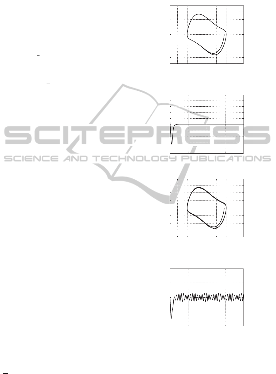
The state response of the closed loop system using the
above state feedback with the same initial condition
of Fig.3 is shown in Fig.5. The state feedback input is
shown in Fig.6. Fig.7 and 8 show the state response
and feedback input of the same closed loop system as
the above with an input disturbance 0.5sin(10t).
[EXAMPLE 2].
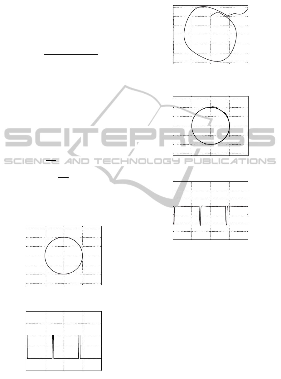
Consider the same system (36) and (37). Here, we
define the desired trajectory by the circle
x
∗
1
(t) = sint
x
∗
2
(t) = cost. (44)
The desired input for this trajectory is
f(u
∗
(t)) = (1 − sin
2
t)cost (45)
This desired state response is shown in Fig.9. Fig.11
shows a disturbed state response when a disturbance
signal described in Fig.10 is added to the desired in-
put (45). The linear time-varying system that approx-
imate this nonlinear system around the desired circle
trajectory is written as follows.
d
dt
∆x
1
(t)
∆x
2
(t)
= A(t)
∆x
1
(t)
∆x
2
(t)
+ b(t)∆u
(46)
−3 −2 −1 0 1 2 3
−3
−2
−1
0
1
2
3
X1
X2
Figure 5: State Response of the Closed Loop with the Initial
Condition near the Limit Cycle.
0 5 10 15 20
−8
−6
−4
−2
0
2
4
6
8
TIME [sec]
INPUT
Figure 6: Feedback Input.
−3 −2 −1 0 1 2 3
−3
−2
−1
0
1
2
3
X1
X2
Figure 7: Disturbed State Response of the Closed Loop with
the Initial Condition near the Limit Cycle.
̻
TIME [sec]
INPUT
Figure 8: Feedback Input.
∆x
1
(t) = x
1
(t)−x
∗
1
(t), ∆x
2
(t) = x
2
(t)−x
∗
2
(t), ∆u(t) =
u(t) − u
∗
(t) where , x
∗
1
(t), x
∗
2
(t) and u
∗
(t) are defined
in (44) and (45). From (34), A(t) and b(t) become as
follows.
ICINCO2013-10thInternationalConferenceonInformaticsinControl,AutomationandRobotics
414
A(t) =
0 1
−1+ 2x
∗
1
(t)x
∗
2
(t) −1+ x
∗2
1
(t))
b(t) =
0
ν(t)
(47)
where
ν(t) =
2exp(−0.5u
∗
(t))
(1+ exp(−0.5u
∗
(t))
2
(48)
From the above, the controllability matrix U
c
(t) be-
comes
U
c
(t) = ν(t)
0 1
1 x
∗2
1
(t) − 1
(49)
which implies that the system is controllable. Then,
if we define λ(t) = ν(t), c
T
0
(t), c
T
1
(t) and c
T
2
(t) can be
chosen as the same functions as in (41) with x
∗
(t) in
(44). Using the same desired closed loop character-
istic polynomial defined in (42), the pole placement
state feedback is obtained as follows.
∆u(t) = −
1
ν(t)
(5+ 2x
∗
1
(t)x
∗
2
(t))∆x
1
(t)
−
1
ν(t)
(4+ x
∗2
1
(t))∆x
2
(t) (50)
Fig.12 shows the state responce of the closed loop
system with the same disturbance. Its initial condi-
tion is on the desired trajectory. The state feedback
input is shown in Fig.13.
−2 −1 0 1 2
−1.5
−1
−0.5
0
0.5
1
1.5
X1
X2
Figure 9: Desired Trajectory.
0 5 10 15 20
−0.5
0
0.5
1
1.5
2
TIME [sec]
Disturbance
Figure 10: Disturbance Input Signal.
̻ ̻
̻
̻
̻
;
;
Figure 11: Disturbed State Response with the Initial Condi-
tion on the Desired Trajectory.
−2 −1 0 1 2
−1.5
−1
−0.5
0
0.5
1
1.5
X1
X2
Figure 12: State Response of Stabilization of Limit Cycle.
̻
̻
̻
̻
TIME [sec]
INPUT
Figure 13: State Response of Stabilization of Limit Cycle.
4 CONCLUSIONS
This paper concerned the problem of stabilization of
some desired trajectory of nonlinear systems. Nonlin-
ear system can be approximated using a linear time-
varying system around this trajectory. The author al-
ready proposed the simple design procedure of the
pole placement controller for linear time-varying sys-
tem. The paper showed that this design method can be
applied to the trajectory stabilization control of non-
linear systems.
REFERENCES
Chi-Tsong Chen (1999)C Linear System Theory and Design
(Third edition). OXFORD UNIVERSITY PRESS
StabilizationofaTrajectoryforNonlinearSystemsusingtheTime-varyingPolePlacementTechnique
415

Charles C. Nguyen (1987)C Arbitrary eigenvalue assign-
ments for linear time-varying multivariable control
systems. International Journal of Control, 45–3, 1051–
1057
W. J. Rugh (1993) Linear System Theory 2nd Edition pren-
tice hall
Y. Mutoh (2011)C A New Design Procedure of the Pole-
Placement and the State Observer for Linear Time-
Varying Discrete Systems. Informatics in Control, Au-
tomation and Robotics, p.321-334, Springer
Michael Val´aˇsek (1995)C Efficient Eigenvalue Assignment
for General Linear MIMO systems. Automatica, 31–
11, 1605–1617
Michael Val´aˇsek, Nejat Olgac¸ (1999)C Pole placement
for linear time-varying non-lexicographically fixed
MIMO systems. Automatica, 35–1, 101–108
Y. Mutoh and Kimura (2011)C Observer-Based Pole Place-
ment for Non-Lexicographically-fixed Linear Time-
Varying Systems. 50th IEEE CDC and ECC
ICINCO2013-10thInternationalConferenceonInformaticsinControl,AutomationandRobotics
416
