Agent based Simulations of Epidemics on a Large Scale

Toward the Right Choice of Parameters

∗

Robert Els

asser

, Adrian Ogierman

and Michael Meier

Department of Computer Sciences, University of Salzburg, A-5020 Salzburg, Austria

Institute for Computer Science, University of Paderborn, 33102 Paderborn, Germany

Keywords:

Epidemic Algorithms, Power Law Distribution, Disease Spreading, Public Health.

Abstract:

In a world where epidemic outbreaks may take many lives, forecasting and analysis tools are of high impor-

tance - for an urban area such as New York City, a continent like Africa, as well as for the world itself. Such

tools provide valuable insight on different levels and help to establish and improve embankment mechanisms.

In this paper, we present an agent-based algorithmic framework to simulate the spread of epidemic diseases.

Based on the population structure of Germany, we investigate the impact of the number of agents, representing

the population, on the quality of the simulation. Real world data provided by the Robert Koch Institute (Ar-

beitsgemeinschaft Inﬂuenza, 2011; Robert Koch Institute, 2012) is used to evaluate our results. In a second

step we empirically analyze the effects of certain non-pharmaceutical countermeasures as applied in the USA

against the Inﬂuenza Pandemic in 1918-1919 (Markel et al., 2007). Our simulation and evaluation tool par-

tially relies on the probabilistic movement model presented in (Els

asser and Ogierman, 2012). Based on our

empirical tests, we conclude that the amount of agents in use can have a huge impact on the accuracy of the

achieved simulation results. This reveals several challenges, which have to be taken into account in the design

of forecasting and analysis tools for the spread of epidemics. On the other hand, we show that by utilizing the

right parameters in our algorithmic framework - some of them being obtained from real world observations

(Eubank et al., 2004) - one can efﬁciently approximate the course of a disease in real world.

1 INTRODUCTION

In order to improve our chances to control an epi-

demic outbreak, we need proper models which de-

scribe the spread of a disease. Institutes, govern-

ments, and scientists all over the world work inten-

sively on forecasting systems to be well prepared if

an unknown disease appears.

In recent years a huge amount of theoretical and

experimental study has been conducted on this topic.

While theoretical analysis provides important and

sometimes even counter intuitive insights into the

behavior of an epidemic (e.g. (Borgs et al., 2010;

Els

asser and Ogierman, 2012)), in an experimental

study one can take many different settings and pa-

rameters (Lee et al., 2008; Lee et al., 2010) into ac-

count. These usually cannot be considered simul-

taneously in a mathematical framework. A speciﬁc

topology, for example, may have its own attributes

∗

Partially supported by the Austrian Science Fund

(FWF) under contract P25214 and by DFG project SCHE

1592/2-1.

that are completely different in other topological set-

tings. Small islands connected only by ferries obvi-

ously offer other spreading opportunities than a huge

metropolitan city. Furthermore, the characteristics of

the spread of an epidemic also depend on the behav-

ior of the infected individuals. That is, different peo-

ple spread the disease (in its early stage) in different

ways, which may or may not lead to an outbreak.

The goal of this paper is to present and empiri-

cally analyze a new dynamic model for the spread of

epidemics. One of our objectives is to ﬁnd the right

parameters, which lead to realistic settings. There-

fore, we investigate a general simulation environment,

in which the different parameters can easily be ad-

justed to real world observations. A second objec-

tive is to evaluate similarities between countermea-

sure approaches in our model and the real world. We

use empirical data for the comparison. Our tool is

agent-based, i.e., the individuals (or groups of such)

are modeled by agents interacting with each other.

The environment approximates the geography of Ger-

many, in which agents may travel between cities.

263

Elsässer R., Ogierman A. and Meier M..

Agent based Simulations of Epidemics on a Large Scale - Toward the Right Choice of Parameters.

DOI: 10.5220/0004429402630274

In Proceedings of the 3rd International Conference on Simulation and Modeling Methodologies, Technologies and Applications (SIMULTECH-2013),

pages 263-274

ISBN: 978-989-8565-69-3

 2013 SCITEPRESS (Science and Technology Publications, Lda.)

Within a city the agents interact according to the prob-

abilistic model presented in (Els

asser and Ogierman,

2012) in a distributed manner. For a detailed descrip-

tion of the algorithmic framework see Section 2.

1.1 Related Work

There is a huge amount of work focusing on the anal-

ysis of epidemic diseases. In this subsection we pro-

vide an overview of the results which are closely re-

lated to the topic of this paper. In our description, we

often rely on the style and wording of (Els

asser and

Ogierman, 2012).

The structure of this subsection is as follows. At

the beginning we present a simple model, which is of-

ten used to simulate an epidemic. Then, we describe

some movement models, on which several studies

w.r.t. the spread of epidemics are based. We conclude

the section by providing an overview of certain em-

pirical results in the ﬁeld of disease spreading as well

as of the main approaches one can identify.

There is plenty of work considering epidemio-

logical processes in different scenarios and on var-

ious networks. The simplest model of mathemati-

cal disease spreading is the so called SIR model (see

e.g. (Hethcote, 2000; Newman, 2003)). The popula-

tion is divided into three categories: susceptible (S),

i.e., all individuals which do not have the disease yet

but can become infected, infective (I), i.e., the individ-

uals which have the disease and can infect others, and

recovered (R), i.e., all individuals which recovered

and have permanent immunity (or have been removed

from the system). Most papers model the spread of

epidemics using a differential equation based on the

assumption that any susceptible individual has uni-

form probability β to become infected from any in-

fective individual. Furthermore, any infected player

recovers at some stochastically constant rate γ.

This traditional (fully mixed) model can easily be

generalized to a network. It has been observed that the

corresponding process can be modeled by bond per-

colation on the underlying graph (Grassberger, 1983;

Newman, 2002). Interestingly, for certain graphs

with a power law degree distribution, there is no

constant threshold for the epidemic outbreak as long

as the power law exponent is less than 3 (Newman,

2003) (which is the case in most real world networks,

e.g. (Faloutsos et al., 1999; Adamic and Huberman,

2000; Amaral et al., 2000; Ripeanu et al., 2002)).

If the network is embedded into a low dimensional

space, or has high transitivity, then there might exist

a non-zero threshold for certain types of correlations

between vertices (Newman, 2002). However, none of

the papers above considered the dynamic movement

of individuals, which seems to be the main source of

the spread of diseases in urban areas (Eubank et al.,

2004).

In (Eubank et al., 2004) the physical contact pat-

terns are modeled by a dynamic bipartite graph, which

results from movement of individuals between spe-

ciﬁc locations. The graph is partitioned into two parts.

The ﬁrst part contains the people who carry out their

daily activities moving between different locations.

The other part represents the various locations in a

certain city. There is an edge between two nodes, if

the corresponding individual visits a certain location

at a given time. Obviously, the graph changes dynam-

ically at every time step.

In (Eubank et al., 2004; Chowell et al., 2003) the

authors analyzed the corresponding network for Port-

land, Oregon. According to their study, the degrees

of the nodes describing different locations follow a

power law distribution with exponent around 2.8

For many epidemics, transmission occurs between in-

dividuals being simultaneously at the same place, and

then people’s movement is mainly responsible for the

spread of the disease.

The authors of (Els

asser and Ogierman, 2012)

considered a dynamic epidemic process in a certain

(idealistic) urban environment incorporating the idea

of attractiveness based distributed locations. The epi-

demic is spread among n agents, which move from

one location to another. In each step, an agent is as-

signed to a location with probability proportional to

its attractiveness. The attractiveness’ of the locations

follow a power law distribution (Eubank et al., 2004).

If two agents meet at some location, then a possible

infection may be transmitted from an infected agent

to an uninfected one. The authors obtained two re-

sults. First, if the exponent of the power law distribu-

tion is between 2 and 3, then at least a small (but still

polynomial) number of agents remains uninfected and

the epidemic is stopped after a logarithmic number of

rounds - even if each agent may spread the disease

for f (n) time steps (where f (n) = o(log n)). Sec-

ondly, if the power law exponent is increased to some

large constant, which is argued to be an implication

of certain countermeasures against the spreading pro-

cess, then the epidemic will only affect a polyloga-

rithmic number of agents and the disease is stopped

after (loglogn)

O(1)

steps. In this case each agent is

allowed to spread the disease for a number of time

steps, which is bounded by some large constant. The

results explain possible courses of a disease and point

out why cost-efﬁcient countermeasures may reduce

In (Eubank et al., 2004) the degree represents the num-

ber of individuals visiting these places over a time period of

24 hours.

SIMULTECH2013-3rdInternationalConferenceonSimulationandModelingMethodologies,Technologiesand

Applications

264

the number of total infections from a high percentage

of the population to a negligible fraction.

In addition to the theoretical papers described

above, plenty of simulation work has also been

done. Two of the most popular directions are the

so called agent-based and structured meta-population-

based approach, respectively (cf. (Ajelli et al., 2010;

Jaffry and Treur, 2008)). Both models have their ad-

vantages and weaknesses. The main idea of the meta-

population approach is to model whole regions, e.g.

georeferenced census areas around airport hubs (Bal-

can et al., 2009), and connect them by a mobility net-

work. Then, within these regions the spread of epi-

demics is analyzed by using the well known mean

ﬁeld theory.

The agent-based approach models individuals

with agents in order to simulate their behavior. In this

context, the agents may be deﬁned very precisely, in-

cluding e.g. race, gender, educational level, etc. (Lee

et al., 2008; Lee et al., 2010), and thus provide a huge

amount of detailed data conditioned on the agents set-

ting. Furthermore, these kinds of models are also able

to integrate different locations like schools, theaters,

and so on. Thus, an agent may or may not be infected

depending on his own choices and the ones made by

agents in his vicinity. The main issue of the agent-

based approach is the huge amount of computational

capacity needed to simulate huge cities, continents or

even the world itself (Ajelli et al., 2010). This lim-

itation can be attenuated by reducing the number of

agents, which then entails a decreasing accuracy of

the simulation. In the meta-population approach the

simulation costs are lower, sacriﬁcing accuracy and

some kind of noncollectable data.

To combine the advantages of both systems, hy-

brid environments were implemented (e.g. (Boba-

shev et al., 2007)). The main idea of such systems

is to use an agent-based approach at the beginning

of the simulation up to some point where a suit-

able amount of agents is infected. Then, the sys-

tem switches to a meta-population-based approach.

Certainly, such a system combines the high accuracy

of the agent-based simulations at the beginning of

the procedure with the faster simulation speed of the

meta-population-based approach at stages in which

both systems may provide similar predictions. Here,

the situation to switch between both approaches (in

both directions) is deﬁned by a threshold T describ-

ing a speciﬁc amount of infected agents. In (Boba-

shev et al., 2007), the authors compared average epi-

demic trajectories produced by both approaches and

determined which threshold value (if any) results in

equivalent average trajectories. For certain epidemics,

especially unknown ones, this adjustment may be dif-

ﬁcult or even not feasible at all.

These kind of simulations are also used to investi-

gate the impact of (non-)pharmaceutical countermea-

sures on the behavior of an epidemic. Germann et

al. (Germann et al., 2006) investigated the spread of

a pandemic strain of the inﬂuenza virus through the

U.S. population. They used publicly available 2000

U.S. Census data to identify seven so-called mixing

groups, in which each individual may interact with

any other member. Each class of mixing group is

characterized by its own set of age-dependent prob-

abilities for person-to-person transmission of the dis-

ease. They considered different combinations of so-

cially targeted antiviral prophylaxis, dynamic mass

vaccination, closure of schools and social distancing

as countermeasures in use, and simulated them with

different basic reproductive numbers R

. It turned

out that speciﬁc combinations of the countermeasures

have a different inﬂuence on the spreading process.

For example, with R

= 1.6 social distancing and

travel restrictions did not really seem to help, while

vaccination limited the number of new symptomatic

cases per 10,000 persons from ∼ 100 to ∼ 1. With

= 2.1, such a signiﬁcant impact could only be

achieved with the combination of vaccination, school

closure, social distancing and travel restrictions.

1.2 Our Results

The results of this paper are two-fold. First, we show

that by increasing the number of agents we are able

to signiﬁcantly improve the accuracy of our results in

the scenarios we have tested. This is due to different

phenomena, which are only visible if the amount of

agents in use is large enough. For example, if the

number of agents exceeds a certain value, then the

epidemic manages to keep a speciﬁc (low) amount

of infected individuals over a long time period. Fur-

thermore, the number of agents has to be above some

threshold to allow the epidemic to enter some speciﬁc

areas/cities in the environment we used. Obviously, a

certain amount of agents is also needed to avoid sig-

niﬁcant ﬂuctuations in our results. However, we could

not determine the right threshold for the speciﬁc in-

stances, which certainly depends on the properties of

the simulated environment and the population size.

The second main result of this paper is that by

setting the parameters properly, one can approximate

the effect of some non-pharmaceutical countermea-

sures, which are usually adopted if an epidemic out-

break occurs. This observation is supported by the

empirical study of (Markel et al., 2007). Interest-

ingly, the right choices of parameters in our experi-

ments seem to be in line with previous observations in

AgentbasedSimulationsofEpidemicsonaLargeScale-TowardtheRightChoiceofParameters

265

real world (e.g. the right power law exponent seems to

be in the range 2.6-2.9, cf. (Eubank et al., 2004)). To

analyze the effect of the countermeasures mentioned

above, we integrate the corresponding mechanisms

on a smaller scale, and then verify their impact on a

larger scale too.

2 THEORETICAL MODELS AND

ALGORITHMIC FRAMEWORK

Our model is based on the distributed algorithmic

framework introduced in (Els

asser and Ogierman,

2012). In that paper a (rough) asymptotic analysis

of the spread of a disease in a large urban environ-

ment was considered, while in our paper we include

its spread on a larger scale with several hundred cities,

and provide a more precise (empirical) analysis on a

smaller as well as on a larger scale. Hereby, the cities

are chosen from a list in descending order of their

population size. Since we do not consider cities in-

habiting less than one agent on expectation, the num-

ber of agents is the limiting factor here. It is intu-

itively clear that large (and thus attractive) cities play

a major role in a fast spread of an epidemic since a

higher population density entails a potentially higher

infection probability. Excluding such hotspots would

of course slow down the infection spread. The prob-

lem is, this could only be achieved by quarantine the

whole city itself. One cannot assume inhabitants liv-

ing and working there would or could leave every-

thing behind. Therefore we consider such strategies

only on a smaller scale.

In our model, the agents may not only move be-

tween locations within a city but between cities as

well. Furthermore, due to simplicity the agents are

not categorized (i.e., they do not provide further prop-

erties like gender etc.). Note, we are not interested in

the evaluation of such details. In the following, we

brieﬂy introduce the model.

Environment and Movement. Our model incorpo-

rates both intra- and inter-city movement. We model

the inter-city movement using a complete graph G =

(V,E). In this graph, each c ∈ V corresponds to a city

of Germany. However, depending on the size, not ev-

ery city is contained in V . The population is repre-

sented by n =

∑

c∈V

agents, with n

being the number

of agents assigned to c proportional to its real world

population. Furthermore, each city contains a num-

ber of so called cells described below. Agents may

move independently from one cell to another or even

travel to another city in each step. Each city c ∈ V is

assigned an attractiveness d

proportional to its pop-

ulation size (w.r.t. the whole population). Note, after-

wards d

does not change anymore. Let A

i,s,t

be the

event that agent i travels from city s to t. Let further

p be the probability that an agent decides to travel

at all, and let dist(s,t) be the Euclidean distance be-

tween cities s and t. Then, the probability that event

i,s,t

occurs is given by

Pr(A

i,s,t

) = p ·

· dist

−1

(s,t)

∑

(s, j)∈E

· dist

−1

(s, j)

Thus, the probability for an agent entering a speciﬁc

city is governed by the distance to said city, its popu-

lation size as well as the current position of the con-

sidered agent.

Since our model incorporates intra-city movement

as well, each c ∈ V is a clique of cells on its own.

These cliques are deﬁned by G

= (V

) with κn

being the size of V

(recall that n

is the number of

agents assigned to city c). Note, κ does not affect the

amount of agents but the amount of cells only. The

nodes v ∈ V

are the cells described above. Here,

κ > 0 is a constant, which will be speciﬁed in the

upcoming experiments. The cells represent locations

within a city an agent can visit. Each cell may contain

agents (individuals), depending on the cells so called

attractiveness. The attractiveness d of a cell v is cho-

sen randomly with probability proportional to 1/d

where α > 2 is a constant depending on the simu-

lation run. In each step, if an agent decides not to

visit another city, then it moves to a randomly chosen

cell according to the distribution of the attractiveness’

among the cells. This also holds for the ﬁrst cell an

agent is accommodated in after entering a city.

Epidemic. We use three different states to model

the distributed spreading process. These states par-

tition the set of agents into three groups; I ( j) con-

tains the infected agents in step j, U( j) contains the

uninfected (susceptible) agents in step j, and R ( j)

contains the resistant agents in step j. Whenever

it is clear from the context, we simply write I , U,

and R , respectively. If at some step j an uninfected

agent i visits a cell (within a city) which also contains

agents of I ( j), then i becomes infected with proba-

bility 1 − (1 − γ)

( j)

, with I

( j) being the number of

infected individuals in the same cell. We refer to the

concrete value of γ in the upcoming simulations.

Countermeasures. In our model, the countermea-

sures are governed by the parameters α and κ. That

is, high values of these two parameters imply a high

SIMULTECH2013-3rdInternationalConferenceonSimulationandModelingMethodologies,Technologiesand

Applications

266

level of countermeasures and vice-versa. With coun-

termeasures applied, individuals avoid places with a

large number of persons more often, waive needless

tours, and are more careful when meeting other peo-

ple. While α is mostly responsible for a decreas-

ing number of visitors within a cell, and thus for the

avoidance of crowded areas for example, κ governs

the total space available for all individuals. That is,

if κ increases, then more cells are available for the

total number of individuals, and meetings within the

same cell are less frequent. Thus, κ basically mod-

els how careful people interact with each other when

they meet. As pointed out in (Markel et al., 2007),

a single countermeasure alone is most likely not suf-

ﬁcient to stop an epidemic. Therefore, we assume a

combination of countermeasures to be in place, which

then would be able to sufﬁciently inﬂuence the pa-

rameters α and κ. Although the models described

above already provide everything needed to simulate

the use of countermeasures, one aspect is still miss-

ing. When do we activate/deactivate the countermea-

sures and what order of magnitude should they have?

We use two different types of countermeasure-models

for this purpose: a (multi-tier) level based approach

considering the amount of infected agents in the cur-

rent step, and a ratio based approach considering the

amount of newly infected agents in the current step

compared to the one in the step before. In the follow-

ing, we use α

and κ

as initial values for α and κ,

respectively.

In the level based model, we have one or more

levels, and within each level a certain pair of param-

eters α and κ is used. Let LM

stand for the level

based model with m levels L = {l

,...,l

} ∪ l

. Fur-

ther, let T = {l

,..., l

} be the set deﬁning

the transition points for all levels, i.e., l

deﬁnes the

transition point from level i to i − 1 whereas l

de-

ﬁnes the transition point from level i to i + 1. Note,

= l

i+1

does not necessarily hold. Additionally,

,α

,...,α

and κ

,κ

,...,κ

deﬁne the parameters

α and κ, which are applied in the corresponding levels

,. .. ,l

. For example, model LM

uses 2 levels. Let

us assume that l

= 0, l

= l

= 10, l

= l

= 20, l

∞. That is, if at most 10 percent of the population

of a city is infected in step i, α

and κ

are applied

to simulate the spread of the disease. If the num-

ber of infected individuals is larger than 10 percent,

then α

and κ

are used. Should the amount of infec-

tions go even above 20 percent, both parameters are

raised to α

and κ

, respectively. Similarly, both pa-

rameters are lowered to the previous values whenever

the amount of infections falls below the correspond-

ing transition values.

In contrast, the ratio based model RM uses a non

static approach. Let the set of newly infected nodes of

a city c in step i be denoted by I

∗

(i). Furthermore, let

and κ

denote the corresponding parameters used

in step i. If

∗

(i)|

∗

(i−1)|

≥ a, for some constant a, then

we set α

i+1

= α

+ z

and κ

i+1

= κ

+ z

, where z

are some small constants which will be speciﬁed later.

Consequently, if

∗

(i)|

∗

(i−1)|

≤ 1/a, then we set α

i+1

max{α

,α

− z

} and κ

i+1

= max{κ

,κ

− z

}. The

values applied in the various models are speciﬁed in

Section 3.5.

3 EXPERIMENTAL ANALYSIS

As already stated in Section 1, the environment ap-

proximates the geography of Germany with up to 10

million agents. Note, the obtained results are almost

identical for the same simulations utilizing 100 mil-

lion agents. Depending on the number of agents, our

simulations use several hundred cities as visitable ar-

eas spread all over the country. Each city is assumed

to be reachable from any other city. However, an

agent may travel at most 1000 km within a single time

step. Each time step represents a whole day in the real

world. Consequently, an agent moving from one city

to another has to wait until its destination is reached

before it can interact with other agents at its destina-

tion.

3.1 Setup and Implementation

The experiments, including the ones with 100 mil-

lion agents, were mostly performed on a computa-

tion node of the Doppler cluster at the University of

Salzburg. This node integrates a quad-socket AMD

Opteron 6274 CPU (16 physical cores at 2.1 GHz

each) with 512 GB RAM (32 x 16GB DIMMs). An

Intel Xeon E5430 CPU (2,66 GHz, 4 physical cores)

has been used as a secondary evaluation unit for ex-

periments which were not so critical in terms of time.

Our simulator is implemented in Java and uses

an agent-based core architecture, where each agent,

depending on the number of overall agents in use,

represents several inhabitants during the simulation.

Furthermore, our system is completely event driven.

Overall we are able to perform large scale experi-

ments with more than 100 million agents in a reason-

able time frame. Since such huge amounts of agents

generate a signiﬁcant impact in terms of performance,

several parallelization approaches are implemented.

For example, several worker threads are used, which

are chosen accordingly to the number of available

physical cores.Furthermore, to decrease the compu-

AgentbasedSimulationsofEpidemicsonaLargeScale-TowardtheRightChoiceofParameters

267

tational time for inter-city travels, we also take ad-

vantage of a parallelization approach concerning the

agents themselves.

3.2 Simulations

In the upcoming sections we present and evaluate our

results. Due to space limitations, only a selection of

the results is presented here. In the following we fo-

cus on

1. the impact of the number of agents on the char-

acteristics of the simulated epidemic compared to

real world data, and

2. the impact of non-pharmaceutical countermea-

sures on the behavior of the epidemic (e.g. social

distancing, school closures, and isolation (Markel

et al., 2007)).

Furthermore, we also analyze our parameter set-

tings. Although this is only a short part, our settings

seem to coincide with the real world observations of

(Eubank et al., 2004), and thus provide an additional

valuable insight. Note that the ﬁgures presented in

this section show values based on the real world pop-

ulation size and not on the number of agents. Thus,

a direct comparability is given without the need to

scale.

3.3 Relevance of the Chosen Parameters

Based on real world observations (e.g. (Eubank et al.,

2004)), we chose α = 2.8 and κ = 1 as a starting point

for a series of simulations concerning α and κ, re-

spectively. Each plot represents values averaged over

50 different simulation runs for each parameter con-

stellation utilizing 10 million agents. The parameter

notation is given in Table 1.

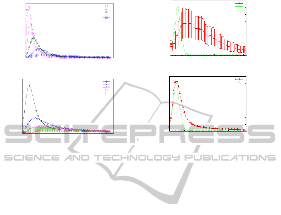
In Figure 1(a) and 1(b) we analyze the impact of

α and κ on the behavior of the epidemic, and compare

the results to the characteristics of a typical Inﬂuenza

case reported by the RKI

. To increase the readabil-

ity, we omit to add the RKI-plot as the 6th one. In-

stead we refer the reader to Fig. 2. Note, although

the plots for α = 2.4 and α = 2.6 may seem more

similar to the RKI-curve at ﬁrst sight, the differences

to the RKI-plot (cf. Table 2 for an example of simi-

larity measures) are signiﬁcant when scaled properly.

Besides, of all ﬁve α-values α = 2.8, which has also

been obtained in (Eubank et al., 2004) in a different

context, represents the best tradeoff between curve

similarity and amount of infections. All remaining

parameters were set to identical values as in Case 1

(cf. Section 3.4). For κ a similar phenomenon can be

observed. With increasing κ (including fractional val-

ues), the characteristics of the curve (i.e., the amount

Table 1: The parameter notation used in the evaluation.

γ With this probability an agent v ∈ U is being

infected independently by each w ∈ I occu-

pying the same cell at the same time.

↑

The amount of steps an agent v ∈ I is infec-

tious, thus being able to infect others.

City

init

Initial amount of cities the infection is being

placed in.

Agent

init

Amount of initially infected agents which

are placed in City

init

different cities.

α The power law exponent used to compute

the attractiveness of the cells within each

city.

κ A multiplicative factor to increase/decrease

the amount of cells proportional to the ini-

tially assigned amount of agents. With κ = 1

the amount of agents is identical to the num-

ber of cells within each city.

of infected individuals at the peak vs. total number of

infections and total duration of the outbreak) become

less and less accurate. Even if we increase the value

to 2, the obtained curve does not follow the charac-

teristics of the real world observations reported by the

RKI

anymore.

In terms of the probability of infection γ we sim-

ply chose a reasonable value low enough to model an

Inﬂuenza epidemic, but high enough to provoke an

outbreak. This seemed reasonable due to the (at least

to our knowledge) lack of concrete values deduced

from real world observations.

3.4 Case 1 - Number of Agents

Before we present the results for this case, we ﬁrst in-

troduce the relevant sources for comparison. For Sub-

case a), we compare our results to real world data pro-

vided by the RKI (Robert Koch Institute, 2012) Surv-

Stat system for the year 2007. The parameter values

were taken from reference data provided by the RKI

(Arbeitsgemeinschaft Inﬂuenza, 2011) where possi-

ble, or set to reasonable ones otherwise. In Subcase

b) then, a disease for a ﬁctional epidemic is presented.

3.4.1 RKI: Basis of Comparison

In this case, we compare our results to the real world

data provided by the RKI

. For this purpose we use

two different data sources: the ofﬁcial report of the

The Robert Koch Institute (RKI) is the central fed-

eral institution in Germany responsible for disease con-

trol and prevention and is therefore the central fed-

eral reference institution for both, applied and response-

orientated research. (Source: http://www.rki.de/EN/Home/

homepage node.html)

SIMULTECH2013-3rdInternationalConferenceonSimulationandModelingMethodologies,Technologiesand

Applications

268

2e+06

4e+06

6e+06

8e+06

1e+07

1.2e+07

1.4e+07

1.6e+07

1.8e+07

0 10 20 30 40 50

Newly Infected Inhabitants

Week

alpha 2.4

alpha 2.6

alpha 2.8

alpha 3.0

alpha 3.2

(a) 2.4 ≤ α ≤ 3.2

1e+06

2e+06

3e+06

4e+06

5e+06

6e+06

7e+06

8e+06

0 10 20 30 40 50

Newly Infected Inhabitants

Week

kappa 1.0

kappa 2.0

kappa 3.0

kappa 4.0

kappa 5.0

(b) 1 ≤ κ ≤ 5

Figure 1: A composition of some simulation runs concern-

ing varying α (1(a)) and κ (1(b)) only. All other parameters

are identical to Case 1 (cf. Section 3.4). Each result rep-

resents the average of 50 different simulation runs with 10

million agents for the topology of Germany.

Inﬂuenza epidemiology of Germany for 2010/2011

(Arbeitsgemeinschaft Inﬂuenza, 2011) and an online

database containing obligatory reports called SurvS-

tat (Robert Koch Institute, 2012).

Relevance. The data for the SurvStat database and

the report of 2010/2011 itself were obtained from

more than 1% of all primary care doctors spread all

over Germany. Note that not every infected person

consults a doctor, which implies that the data of the

SurvStat system contains only the serious courses

of the disease. Nonetheless, these sources provide

a valuable tool to obtain insight into the spread

and persistence of the Inﬂuenza virus in Germany.

Further, due to the data’s signiﬁcance, it is possible

to estimate the number of infections within certain

areas as well. Since the spread of infections in the

real world is inﬂuenced by factors like seasonal

ﬂuctuations or the virus’ aggressiveness, the number

of total infections may signiﬁcantly differ from

year to year, cf. (Robert Koch Institute, 2012) for

different years. However, the course of the curve

usually does not change. Consequently, we do

not focus on absolute values in our simulations,

but on the characteristics of our results. These

characteristics remain, up to some scaling factor,

identical over the whole data set provided by the RKI.

100000

200000

300000

400000

500000

600000

0 10 20 30 40 50

500

1000

1500

2000

2500

3000

3500

4000

Newly Infected Inhabitants(Simulation)

Newly Infected Inhabitants(RKI Data)

Week

Simulation

SurvStat 2007

(a) 10.000 Agents

1e+06

2e+06

3e+06

4e+06

5e+06

6e+06

0 10 20 30 40 50

500

1000

1500

2000

2500

3000

3500

4000

Newly Infected Inhabitants(Simulation)

Newly Infected Inhabitants(RKI Data)

Week

Simulation

SurvStat 2007

(b) 10.000.000 Agents

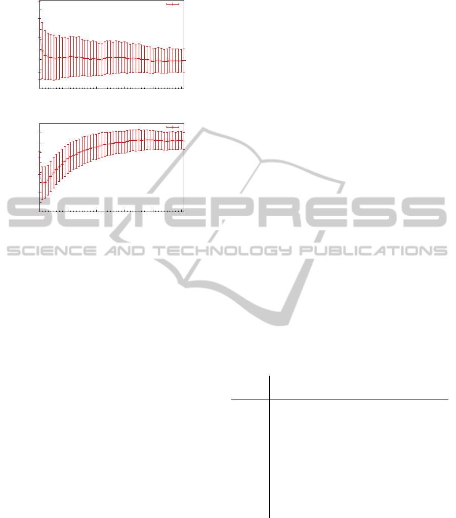
Figure 2: Simulation results for Case 1a) (red) in compar-

ison to real world data (green) provided by the RKI for a

varying amount of agents. Each result represents the av-

erage of 50 different simulation runs. The reliability of the

averaged value is indicated by the corresponding conﬁdence

interval.

3.4.2 Subcase a)

The Parameters in this case are as follows. We set

γ = 7%, D

↑

to 5 days, the amount of initially infected

cities City

init

to 1 (namely Berlin), and the amount of

initially infected agents Agent

init

to 0.0015% of the

overall agents used for these simulations. Further-

more, α = 2.8 and κ = 1.

Each obtained plot represents the average of 50

different simulation runs. Figure 2 shows the results

for the ﬁrst subcase. Here, the green curve represents

the real world data provided by the RKI for the year

2007 while the red curve represents our simulation re-

sults. Note that both curves vary signiﬁcantly in terms

of absolute numbers. However, this is not our focus

here. Due to the level of abstraction in our model and

since the RKI data only contains reported cases (see

above), the absolute numbers do not coincide. Addi-

tionally, as stated above, the data provided by the RKI

also differs signiﬁcantly (in terms of absolute num-

bers but not the disease characteristics) from year to

year (cf. (Robert Koch Institute, 2012)). Therefore,

we focus on the course of the disease and the result-

ing characteristics of the plotted curves.

It is easy to see that the more agents are used, be-

ginning from Figure 2(a) up to Figure 2(b), the more

the curve characteristics converge. Moreover, the ac-

AgentbasedSimulationsofEpidemicsonaLargeScale-TowardtheRightChoiceofParameters

269

curacy of each simulation run increases as well (cf.

the conﬁdence intervals in Figure 2). With at least

500.000 agents in use, both curves become similar.

Note that we shifted the outbreak position of the RKI

data to the origin to create a comparable situation.

Since the moment of an outbreak varies in reality as

well (cf. (Robert Koch Institute, 2012)) and the be-

ginning of the disease is not important for us, this re-

location does not have any inﬂuence on the data or the

evaluation itself.

To obtain a more formal evaluation, we deﬁne

three measures, which are used to compare our results

to the data provided by the RKI. These are: the time

to peak (TTP), the epidemic duration (ED), and the

area of the curve (AC). The time to peak describes the

week with the maximum amount of newly infected

agents of the corresponding curve. The area of the

curve is simply the summation of the area between the

origin and the endpoint EP (deﬁned by the epidemic

duration). Finally, the endpoint of the epidemic dura-

tion is the week in which only a minor amount of new

infections occur, and no signiﬁcant new infections are

observed anymore. Minor infections are deﬁned to

start at a step i and last till the last step j of the sim-

ulation while for all steps i ≤ i

≤ j it holds that the

amount of newly infected agents does not exceed 9%

of the maximum value.

In Table 2 we consider the relative values of these

measurements compared to the RKI data. That is,

the numbers given in this table represent the ratio be-

tween the value obtained in our simulations and the

value provided by the RKI. For example, a value of

4.00 for TTP in the case of 10.000 agents implies that

the time to peak in our case divided by the time to

peak in the real world data is 4.

Using the individual deviation measurements, we

deﬁne a global deviation value by the formula

TTP +

· AC +

· ED. For simplicity we consider

each individual measurement uniformly weighted.

The results, which conﬁrm our previous observations,

are given in Table 2 and Figure 3.

All obtained results and previous statements

imply a fragile balance between the accuracy, the

parameter setting, and the amount of agents in use.

3.4.3 Subcase b)

In Contrast to Subcase a), the Epidemic here is a Fic-

tional One. We set γ = 1.5%, D

↑

to 5 days, the amount

of initially infected cities City

init

to 1 (namely Berlin),

and the amount of initially infected agents Agent

init

0.0015% of the overall agents used for these simula-

tions. Furthermore, α = 2.8 and κ = 1.

Table 2: Quantitative comparison and deviation measure-

ments of the achieved results in Case 1a) with respect to the

data provided by the RKI. The results refer to the following

properties: time to peak (TTP), the epidemic dration (ED),

and the area of the curve (AC). Here, the AC is starting at

the origin and ending at the endpoint EP deﬁned by the ED.

All values are given as a relative deviation concerning the

data provided by the RKI. The deviation value itself is com-

puted utilizing

· TTP +

· AC +

· ED.

Deviation

Agents TTP

ED /

(week)

Deviation

Value

10 K 2,33 3,53/53 5,58 3,81

25 K 2,00 3,53/53 4,71 3,41

50 K 1,83 3,47/52 3,70 3,00

100 K 1,33 2,87/43 3,10 2,43

250 K 1,17 2,27/34 2,59 2,01

500 K 1,17 1,87/28 2,29 1,77

1 M 1,17 1,67/25 2,16 1,66

2.5 M 1,00 1,53/23 2,00 1,51

5 M 1,00 1,47/22 1,92 1,46

10 M 1,00 1,40/21 1,88 1,43

10K 25K 50K 100K 250K 500K 1M 2.5M 5M 10M

Deviation measure

Simulation runs to the corresponding agent numbers

TTP

Deviation value

Figure 3: A visual representation of the data of Table 2.

In this subcase, we chose γ relatively low com-

pared to the subcase above to emphasize the distor-

tion. We show a signiﬁcantly varying course of dis-

ease, which even exceeds the distortion of Subcase a).

Using these parameters we were able to identify mul-

tiple curve characteristics, partially shown in Figure

4. The differences are signiﬁcant. First, we observed

the extinction of the disease almost instantly after the

outbreak, followed by a completely unpredictable be-

havior including an increasing as well as a decreasing

inﬂuence of the disease, up to a self-stabilizing infec-

tion spreading (cf. Fig. 4(a) and 4(b)). Since no other

parameter was altered, only the different number of

agents could have such a strong inﬂuence on the re-

sults.

Combined, both subcases indicate a signiﬁcant in-

ﬂuence of the amount of agents in use on the spread-

ing process itself. One main goal in such simula-

tions is to gain some speedup with a lower number

SIMULTECH2013-3rdInternationalConferenceonSimulationandModelingMethodologies,Technologiesand

Applications

270

-20000

20000

40000

60000

80000

100000

120000

140000

160000

0 10 20 30 40 50

Newly Infected Inhabitants(Simulation)

Week

Simulation

(a) 100.000 Agents

20000

40000

60000

80000

100000

120000

140000

160000

180000

0 10 20 30 40 50

Newly Infected Inhabitants(Simulation)

Week

Simulation

(b) 10.000.000 Agents

Figure 4: Simulation results for Case 1b) (red) for a varying

amount of agents. Each result represents the average of 50

different simulation runs. The reliability of the averaged

value is indicated by the corresponding conﬁdence interval.

of agents while keeping the collectible data (for ex-

ample the number of infections) almost identical in

terms of accuracy. Now, this seems to be a very fragile

premise which cannot necessarily be achieved. Note,

we did not explicitly tune the settings for the dif-

ferent amount of agents since such possibilities may

not be present or applicable for medical forecasting

and disease estimation systems. Especially for un-

known or largely unexamined diseases this may be

very problematic. However, due to the dependency of

the amount of cells in a city and the amount of agents

in use, this is done, to some extent, implicitly by our

model.

3.5 Case 2 - Non-pharmaceutical

Countermeasures

Now we extend our analysis to incorporate non-

pharmaceutical countermeasures such as school clo-

sures and social distancing. Here, we stick to a ﬁc-

tional epidemic simply because it simpliﬁes the pre-

sentation, i.e., due to the increase of γ to 12%, a faster

spread is achieved and the impact of the used counter-

measures is ampliﬁed. Similar to Case 1, we set D

↑

5 days, the amount of initially infected cities City

init

1 (namely Berlin), and the amount of initially infected

agents Agent

init

to 0.00075% of the overall agents (to

compensate the higher γ at the beginning). All rele-

vant parameters concerning the countermeasure mod-

els can be found in Table 4 and 5.

We assume that such countermeasures basically

affect the parameters α and κ, since the individu-

als will most likely avoid places with a large num-

ber of persons, waive needless tours, and be more

careful when meeting other people. Although one

of these modiﬁcations alone is most likely not suf-

ﬁcient (Markel et al., 2007), we can simply assume a

combination of these strategies to be in place, which

then would be able to sufﬁciently inﬂuence α and κ.

For obvious reasons, we cannot compare our simula-

tion results to current real world data, which consider

different epidemics with varying (or no) countermea-

sures in use. Therefore, we use the work of Markel et

al. (Markel et al., 2007) for this purpose. Especially

Figure 5 is of particular interest. There, the direct cor-

relation between establishing countermeasures and a

decreasing amount of new infections (and vice versa)

is well highlighted. We observed an identical effect in

our simulations (cf. Figures 6, 7, 8 and Table 3). Note

that different combinations of countermeasures used

in (Markel et al., 2007) entail different kinds of im-

pacts on the death rates. In contrast, we do not focus

on speciﬁc combinations but on sufﬁcient ones to ac-

tually achieve an immediate impact on the epidemic.

Table 3: Percentage of the overall infected inhabitants (Case

2). Column NOCM represents the percentage of overall in-

fections without any countermeasures in use, whereas the

other columns state the gain compared to the case without

countermeasures for the corresponding level based and ratio

based model, respectively.

Agents

Infected Agents (in percent)

NOCM LM

10k 55,45 40,36 24,38 25, 26 31,93

25k 58.57 16, 72 1,56 15, 18 33,43

50k 76,20 13, 49 21,50 28,40 42, 51

100k 75,08 11, 75 −0.29 16, 50 27,88

250k 81,37 11, 13 18,95 16,38 40, 30

500k 85,77 18, 05 16,15 20,04 39, 26

1M 86,12 1.84 14,53 12,16 37, 41

2,5 M 88,22 12,47 14,66 13,42 35,47

5M 87,39 11, 33 8,50 8,90 29,81

10M 88,06 8, 0 9,30 9, 15 32,08

As already described in Section 2, two different

countermeasure approaches are of main interest for

us: the level based (LM

, LM

and LM

), and the ratio

based (RM), respectively. Both use different mecha-

nisms and parameters to achieve the embankment of

the epidemic. Recall that all transition points in the

level based model are chosen w.r.t. the ratio between

the amount of currently infected individuals and the

population size of the city.

AgentbasedSimulationsofEpidemicsonaLargeScale-TowardtheRightChoiceofParameters

271

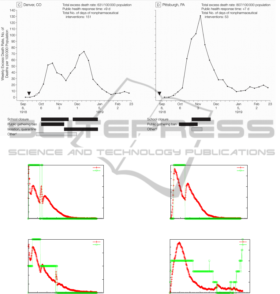
Figure 5: Weekly excess death rates from September 8, 1918, through February 22, 1919 (Markel et al., 2007, Figure 3).

20000

40000

60000

80000

100000

120000

140000

160000

0 50 100 150 200 250 300 350 400

0.2

0.4

0.6

0.8

Infected Inhabitants

Activated Countermeasure Level l

Day

Simulation

Level

(a) Model LM

, 10 million agents

20000

40000

60000

80000

100000

120000

0 50 100 150 200 250 300 350 400

0.5

1.5

Infected Inhabitants

Activated Countermeasure Level l

Day

Simulation

Level

(b) Model LM

, 10 million agents

Figure 6: Example results for BER for Case 2. The number

of agents refers to the total amount in the simulation.

Similar to Case 1, the results with at most 10 mil-

lion agents in use are presented for each model. Al-

though the level based approach is completely dif-

ferent compared to the ratio based approach, the

achieved results are similar. However, the overall in-

crease of α and κ by the ratio based approach may

be noticeably higher, especially if a large number of

10000

20000

30000

40000

50000

60000

70000

80000

0 50 100 150 200 250 300 350 400

0.2

0.4

0.6

0.8

Infected Inhabitants

Activated Countermeasure Level l

Day

Simulation

Level

(a) Model LM

, 10 million agents

5000

10000

15000

20000

25000

30000

35000

0 50 100 150 200 250 300 350 400

Infected Inhabitants

Activated Countermeasure Level l

Day

Simulation

Level

(b) Model RM, 10 million agents

Figure 7: Example results for HAM for Case 2. The number

of agents refers to the total amount in the simulation.

agents is used (cf. for example Figure 8(b)). That is,

while all LM-models use α ≤ 3.3, the RM-model goes

above 4. This implies that the LM-models are more

cost efﬁcient, since both α and κ are kept lower and

therefore less effort is needed to achieve and maintain

said values.

Additionally, to be able to compare our results to

SIMULTECH2013-3rdInternationalConferenceonSimulationandModelingMethodologies,Technologiesand

Applications

272

Table 4: Parameters for the level based countermeasure models relevant for

Case 2.

Level

0 6% 0% 2.8 1.0 4% 0% 2.8 1.0 2% 0% 2.8 1.0

1 ∞ 4% 3.3 1.2 6% 2% 3.1 1.1 4% 1% 3.0 1.0

2 - - - - ∞ 4% 3.3 1.2 6% 2% 3.1 1.1

3 - - - - - - - - ∞ 4% 3.3 1.2

Table 5: Parameters for the ratio based coun-

termeasure model relevant for Case 2.

RM Model

a z

2 0.2 0.1 2.8 1.0

5000

10000

15000

20000

25000

0 50 100 150 200 250 300 350 400

0.5

1.5

2.5

Infected Inhabitants

Activated Countermeasure Level l

Day

Simulation

Level

(a) Model LM

, 10 million agents

1000

2000

3000

4000

5000

6000

0 50 100 150 200 250 300 350 400

Infected Inhabitants

Activated Countermeasure Level l

Day

Simulation

Level

(b) Model RM, 1 million agents

Figure 8: Example results for PB for Case 2. The number

of agents refers to the total amount in the simulation.

the ﬁndings in (Markel et al., 2007), we examine the

following three cities in more detail: BER (population

size: ≈ 3.5 million), HAM (population size : ≈ 1.8

million) and PB (population size: ≈ 146.000). Fig-

ures 6, 7 and 8 represent a composition of some inter-

esting results for each city and model in use. Note

that the green curve in these ﬁgures represents the

countermeasure level for the LM models at the cor-

responding time, and indicates the number of times

have increased α, κ in the RM model. Recall,

in the RM-model level j implies α

= α

∑

k=1

and

= κ

∑

k=1

for a step i.

Our results conﬁrm the impact, inﬂuenced by

the effectiveness of the countermeasures, of different

countermeasures observed in the real world (Markel

et al., 2007). Compared to Figure 5, our simula-

tions show a similar behavior (i.e., more than one

peak during the epidemic). It is easy to see that the

countermeasures presented in (Markel et al., 2007)

directly inﬂuence the course of the epidemic. The

same property can be observed in our results (cf. Fig-

ure 6(b), 7(a) or 8(a)). One can see that depending

on the countermeasure level (indicated by the acti-

vated/used level), the number of infections increases

or decreases. Note that although our ﬁgures show the

number of infected individuals and not the death rate

as shown in Figure 5, a comparison is still possible

since this deviation can be normalized using a scaling

factor.

Furthermore, we observe that small adjustments

of the two parameters α and κ entail a signiﬁcant im-

pact on the number of overall infections (cf. Table 3).

Among others, it was shown that if the power law ex-

ponent (and κ as well) is assumed to be some large

constant, then even a very aggressive epidemic with

γ = 100% will affect no more than a polylogarithmic

number of the population. Our ﬁndings now back up

these observations.

In conclusion, in this case we showed the im-

pact of different countermeasures on the behavior of

a population w.r.t. our model. Although some com-

plexity of the real world is lacking, the similarities

to real world observations are still present. Starting

with settings for the environment, and therefore im-

plicitly the individuals’ behavior, based on real world

observations (cf. Section 3.3) relatively low level

countermeasures were sufﬁcient to embank or at least

signiﬁcantly suppress an outbreak. Essentially the

same properties were already observed in reality (cf.

(Markel et al., 2007)). This underlines the impor-

tance of behavioral and environmental models based

on power law distributions.

4 CONCLUSIONS

Agent based simulators offer various possibilities to

perform very detailed experiments. However, the pa-

rameters used in these experiments highly inﬂuence

the results one might obtain. As we have seen, even

the number of agents has a signiﬁcant impact on the

quality of the results. This includes the reliability of

different simulation runs with an identical parameter

setting. By using the right parameter settings and a

AgentbasedSimulationsofEpidemicsonaLargeScale-TowardtheRightChoiceofParameters

273

proper number of agents, it is possible to approximate

the course of a disease as observed in the real world.

Furthermore, our experiments indicate that the algo-

rithmic framework presented in this paper is able to

describe, to some extent, the impact of certain non-

pharmaceutical countermeasures on the behavior of

an epidemic.

REFERENCES

Adamic, L. A. and Huberman, B. A. (2000). Power-

law distribution of the world wide web. Science,

287(5461):2115.

Ajelli, M., Goncalves, B., Balcan, D., Colizza, V., Hu, H.,

Ramasco, J., Merler, S., and Vespignani, A. (2010).

Comparing large-scale computational approaches to

epidemic modeling: Agent-based versus structured

metapopulation models. BMC Infectious Diseases,

10(190).

Amaral, L. A., Scala, A., Barthelemy, M., and Stanley,

H. E. (2000). Classes of small-world networks. PNAS,

97(21):11149–11152.

Arbeitsgemeinschaft Inﬂuenza (2011). Bericht zur Epi-

demiologie der Inﬂuenza in Deutschland Saison

2010/11.

Balcan, D., Hu, H., Goncalves, B., Bajardi, P., Poletto, C.,

Ramasco, J. J., Paolotti, D., Perra, N., Tizzoni, M.,

den Broeck, W. V., Colizza, V., and Vespignani, A.

(2009). Seasonal transmission potential and activity

peaks of the new inﬂuenza A(H1N1): a Monte Carlo

likelihood analysis based on human mobility. BMC

Medicine, 7:45.

Bobashev, G. V., Goedecke, D. M., Yu, F., and Epstein,

J. M. (2007). A hybrid epidemic model: combining

the advantages of agent-based and equation-based ap-

proaches. In Proc. WSC ’07, pages 1532–1537.

Borgs, C., Chayes, J., Ganesh, A., and Saberi, A. (2010).

How to distribute antidote to control epidemics. Ran-

dom Struct. Algorithms, 37:204–222.

Chowell, G., Hyman, J. M., Eubank, S., and Castillo-

Chavez, C. (2003). Scaling laws for the movement

of people between locations in a large city. Physical

Review E, 68(6):661021–661027.

Els

asser, R. and Ogierman, A. (2012). The impact of the

power law exponent on the behavior of a dynamic epi-

demic type process. In Proc. SPAA’12.

Eubank, S., Guclu, H., Kumar, V., Marathe, M., Srinivasan,

A., Toroczkai, Z., and Wang, N. (2004). Modelling

disease outbreaks in realistic urban social networks.

Nature, 429(6988):180–184.

Faloutsos, M., Faloutsos, P., and Faloutsos, C. (1999). On

power-law relationships of the internet topology. In

SIGCOMM ’99, pages 251–262.

Germann, T. C., Kadau, K., Longini, I. M., and Macken,

C. A. (2006). Mitigation strategies for pandemic in-

ﬂuenza in the United States. PNAS, 103(15).

Grassberger, P. (1983). On the critical behavior of the

general epidemic process and dynamical percolation.

Mathematical Biosciences, 63(2):157 – 172.

Hethcote, H. W. (2000). The mathematics of infectious dis-

eases. SIAM Review, 42(4):599–653.

Jaffry, S. W. and Treur, J. (2008). Agent-Based and

Population-Based Simulation: A Comparative Case

Study for Epidemics. In Louca, L. S., Chrysan-

thou, Y., Oplatkova, Z., and Al-Begain, K., editors,

ECMS’08, pages 123–130.

Lee, B. Y., Bedford, V. L., Roberts, M. S., and Carley, K. M.

(2008). Virtual epidemic in a virtual city: simulat-

ing the spread of inﬂuenza in a us metropolitan area.

Translational Research, 151(6):275 – 287.

Lee, B. Y., Brown, S. T., Cooley, P. C., Zimmerman, R. K.,

Wheaton, W. D., Zimmer, S. M., Grefenstette, J. J.,

Assi, T.-M., Furphy, T. J., Wagener, D. K., and Burke,

D. S. (2010). A computer simulation of employee vac-

cination to mitigate an inﬂuenza epidemic. American

Journal of Preventive Medicine, 38(3):247 – 257.

Markel, H., Lipman, H. B., Navarro, J. A., Sloan, A.,

Michalsen, J. R., Stern, A. M., and Cetron, M. S.

(2007). Nonpharmaceutical Interventions Imple-

mented by US Cities During the 1918-1919 Inﬂuenza

Pandemic. JAMA, 298(6):644–654.

Newman, M. E. J. (2002). Spread of epidemic disease on

networks. Phys. Rev. E, 66(1):016128.

Newman, M. E. J. (2003). The structure and function of

complex networks. SIAM Review, 45(2):167–256.

Ripeanu, M., Foster, I., and Iamnitchi, A. (2002). Mapping

the gnutella network: Properties of large-scale peer-

to-peer systems and implications for system. IEEE

Internet Computing Journal, 6(1):50–57.

Robert Koch Institute (2012). SurvStat@RKI. A web-based

solution to query surveillance data in Germany.

SIMULTECH2013-3rdInternationalConferenceonSimulationandModelingMethodologies,Technologiesand

Applications

274