
Remarks on an Adaptive-type Self-tuning Controller using Quantum
Neural Network with Qubit Neurons
Kazuhiko Takahashi, Yuka Shiotani and Masafumi Hashimoto
Faculty of Science and Engineering, Doshisha University, Kyoto, Japan
Keywords:
Quantum Neural Network, Qubit neuron, Self-tuning Controller, PID Controller, Fuzzy Logic Controller.
Abstract:
This paper presents a self-tuning controller based on a quantum neural network and investigates the con-
troller’s characteristics for control systems. A multi-layer quantum neural network which uses qubit neurons
as an information processing unit is utilized to design an adaptive-type self-tuning controller which conducts
the training of the quantum neural network as an online process. As an example of designing the self-tuning
controller, either a proportional integral derivative controller or a fuzzy logic controller is utilized as a con-
ventional controller for which parameters are tuned by the quantum neural network. To evaluate the learning
performance and capability of the adaptive-type quantum neural self-tuning controller, we conduct computa-
tional experiments to control the single-input single-output non-linear discrete time plant. The results of the
computational experiments confirm both feasibility and effectiveness of the proposed self-tuning controller.
1 INTRODUCTION
Over the past quarter of the century, many studies
conducted worldwide have applied both flexibility
and learning ability of artificial neural networks to
control systems and have proposed many types of
neural-network-based control systems (Hagan et al.,
2002)(Meireles et al., 2003). Neural networks, which
were utilized in a large number of previous stud-
ies in the field of control systems, conduct signal
processing involving real numbers by using a sig-
moid, binary or radial basis function as an informa-
tion processing unit. On the other hand, there are
several advantages to solving classically hard-to-treat,
intractable problems by using real-valued (conven-
tional) neural networks and to providing a new under-
standing of certain brain functions. Therefore, many
studies of hyper-complex numbers neural networks
based on Clifford algebra (Sommer, 2001), such as
complex neural networks whose weights and activa-
tion functions are complex and quaternion neural net-
works developed in hypercomplex quaternion alge-
bra, have been undertaken, and there have been many
successful examples involving the use of such neural
networks in applications requiring spatial processing,
e.g. colour image processing and multiple-dimension
time-series signal processing. Quantum neural net-
works (Ezhov and Ventura, 2000)(Manju and Nigam,
2012), which involvethe introductionof quantum the-
oretical concepts and quantum computing techniques
to neural networks, can also be classified as complex
neural networks because the state of an arbitrary neu-
ron in the quantum neural network is a coherent su-
perposition of multiple quantum states which can be
expressed by complex numbers. A quantum neural
network which utilizes qubit-inspired neurons as in-
formation processing units has been proposed, and its
high learning capability has been confirmed in sev-
eral benchmark tests and applications (Kouda et al.,
2005)(Zhou et al., 2006). As a servo-level controller
application which uses the quantum neural network
with qubit neurons, a direct controller in which the
output of the quantum neural network is the control
input of the object plant has been proposed and its
feasibility demonstrated (Takahashi et al., 2011).
This paper proposes an adaptive-type self-tuning
controller by using a quantum neural network, and in-
vestigates its characteristics for control systems. In
the self-tuning controller, the control input of the
plant is the output from the conventional controller
whose parameters are tuned by the quantum neural
network. Although the self-tuning controller is more
complex than the direct controller, it offers the pos-
sibility of realizing increased robustness. The train-
ing of the quantum neural network can be classi-
fied into two types: online training and offline train-
ing. From the perspective of control applications,
online training, which corresponds to adaptive con-
107
Takahashi K., Shiotani Y. and Hashimoto M..
Remarks on an Adaptive-type Self-tuning Controller using Quantum Neural Network with Qubit Neurons.
DOI: 10.5220/0004425701070112
In Proceedings of the 10th International Conference on Informatics in Control, Automation and Robotics (ICINCO-2013), pages 107-112
ISBN: 978-989-8565-70-9
Copyright
c
2013 SCITEPRESS (Science and Technology Publications, Lda.)

trol, is more practical than offline training, and this
study, therefore, considers the online training of the
quantum neural network. In Section 2, we present
a design of the quantum-neural-network-based self-
tuning controller (hereafter called quantum neural
self-tuning controller), which conducts online train-
ing of the multi-layer quantum neural network with
qubit neurons. In Section 3, computational experi-
ments for controlling a discrete-time non-linear plant
are conducted to evaluate the feasibility of the pro-
posed controller.
2 CONTROLLER DESIGN
Figure 1 shows a schematic of a self-tuning con-
troller for which the control input u(k) is calculated
by a conventional controller for which parameters are
tuned by the quantum neural network. The multi-
layer quantum neural network is designed by combin-
ing qubit neurons in layers. The state of the j-th qubit
neuron in the r-th layer at a sampling number of k can
be given by:
z
r
j
(k) = f(
π
2
δ
r
j
(k) − argv
r
j
(k))
v
r
j
(k) =
∑
i
f(θ
r
i, j
(k)) f(z
r−1
i
(k)) − f (λ
r
j
(k))
. (1)
Here, f(·) is a complex function of the phase which
expresses the qubit state |ψi: f(φ) = e
iφ
(i is an
imaginary unit), δ
r
j
(k) is the reversal parameter cor-
responding to a 2-bit controlled NOT gate, θ
r
i, j
(k) is
the phase parameter corresponding to the phase of a
1-bit rotation gate and λ
r
j
(k) is the threshold parame-
ter. In the input layer (r = I), the network input x
j
(k)
is first converted into the quantum state with a phase
in the range [0,π/2], and then the output, given by
z
I
j
(k) = f((π/2)σ(x
j
(k))), is fed into qubit neurons in
the hidden layer (r = H). Here σ(·) is a sigmoid func-
tion: σ(x) = 1/(1 + e
−x
). The outputs from the qubit
neurons of the hidden and output layers are given by
Eq. (1). By considering the probability of the state in
which |1i is observed from the j-th qubit neuron in
the output layer (r = O), the output from the quantum
neural network u
qnn
j
(k) is defined as follows:
u
qnn
j
(ω(k),x(k)) = |Im(z
O
j
(k))|
2
. (2)
Here, the vector ω(k) is composed of parameters
θ
r
i, j
(k), δ
r
j
(k) and λ
r
j
(k), and the vector x(k) is com-
posed of input x
j
(k). The output from the quantum
neural network u
n
j
(k) is converted from the range
[0,1] into the range [u
min
, u
max
] with a gain factor g
0
j
and shift factor u
qnn
0
j
:
u
n
j
(k) = g
0
j
{u
qnn
j
(ω(k), x(k)) − u
qnn
0
j
}. (3)
Quantum
Neural Network
Plant
u y
Conventional
controller
y
d
+ -
ε
Figure 1: Schematic diagram of the quantum neural self-
tuning controller.
To simplify the quantum neural self-tuning con-
troller’s design, the following single-input single-
output (SISO) discrete-time plant is considered as a
controlling target plant:
y(k+ d) = F(y(k),y(k − 1),· ·· ,y(k − n+ 1),
u(k),u(k− 1), ·· · ,u(k− m− d + 1)), (4)
where y(k) is the plant output, u(k) is the plant in-
put, n and m are the plant orders, d is the dead time
of the plant and F(·) is the function which expresses
plant dynamics. This design makes the following as-
sumptions: the upper limit orders and dead time of
the plant are known. By considering the desired plant
output y
d
(k), the output error ε(k) can be defined by
ε(k) = y
d
(k) − y(k). In this study, the following dig-
ital proportional integral derivative (PID) control law
is utilized as the conventional controller:
u(k) = u(k− 1) + g
T
(k)e(k), (5)
where g(k) = [
K
P
(k) K
I
(k) K
D
(k)
]
T
, in which
K
P
(k), K
I
(k) and K
D
(k) are the proportional
gain, integral gain and differential gain, respec-
tively, e(k) = [
∆ε(k) ε(k) ∆ε(k) − ∆ε(k− 1)
]
T
,
in which ∆ε(k) is the difference of the output error
given by ∆ε(k) = ε(k) − ε(k − 1). The gain parame-
ters are tuned by the output from the quantum neural
network in the quantum neural self-tuning controller.
To define the input vector of the quantum neural
network, the following direct controller which con-
trols the plant represented by Eq. (4) is utilized:
u
d
(k) = F
d
(w(k),x
d
(k)), (6)
where u
d
(k) is the output from the direct controller,
F
d
(·) is the function of the direct controller, the vector
w(k) is composed of the direct controller’s parameters
and x
d
(k) is the input vector of the direct controller,
which is defined as follows:
x
d
(k) = [
y
d
(k+ d) y(k) · ·· y(k− n+ 1)
u(k− 1) ·· · u(k− m − d + 1)
]
T
. (7)
Assuming u(k) − u(k − 1) = u
d
(k) yields
g(k) = {e(k)e
T
(k) + Γ}
−1
e(k)F
d
(w(k),x
d
(k)), (8)
ICINCO2013-10thInternationalConferenceonInformaticsinControl,AutomationandRobotics
108

where Γ = diag(γ
1
,γ
2
,γ
3
), in which γ
i
(i = 1,2,3) is
an arbitrary constant (0 < γ
i
≪ 1). By considering
the right hand side of Eq. (8), the input vector of the
quantum neural network x(k) is defined as follows:
x(k) = [
y
d
(k+ d) y(k) · ·· y(k− n+ 1)
u(k− 1) ·· · u(k− m − d + 1) γ
2
γ
3
∆ε(k)
γ
1
γ
3
ε(k) γ
1
γ
2
{∆ε(k) − ∆ε(k− 1)}
det(e(k)e
T
(k) + Γ)
]
T
. (9)
The training of the quantum neural network is car-
ried out by using a back-propagation algorithm such
that it minimizes the cost function J(k):
ω(k+ 1) = ω(k− d) − η
∂J(k)
∂ω(k− d)
+α∆ω(k− d), (10)
J(k) =
1
2
∑
q
ε
2
q
(k), (11)
where ε
q
(k) = y
d
q
(k) − y
q
(k), ∆ω(k) is the weight in-
crement and η and α are the learning factors. The
gradients of the cost function with respect to the pa-
rameters in the output layer are as follows:
∂J(k)
∂δ
O
j
(k− d)
= −
π
2
g
0
j
∑
q
ε
q
(k)
∑
s
∂ε
q
(k)
∂y
s
(k)
×
∑
t
∂y
s
(k)
∂u
t
(k− d)
∂u
t
(k− d)
∂u
n
j
(k− d)
ξ
j
(k− d),
∂J(k)
∂θ
O
i, j
(k− d)
= g
0
j
∑
q
ε
q
(k)
∑
s
∂ε
q
(k)
∂y
s
(k)
×
∑
t
∂y
s
(k)
∂u
t
(k− d)
∂u
t
(k− d)
∂u
n
j
(k− d)
ξ
j
(k− d)
d
OH
j
(k− d)
×{a
OH
j
(k− d)cos(θ
O
i, j
(k− d) + v
H
i
(k− d))
+b
OH
j
(k− d)sin(θ
O
i, j
(k− d) + v
H
i
(k− d))},
∂J(k)
∂λ
O
j
(k− d)
= −g
0
j
∑
q
ε
q
(k)
∑
s
∂ε
q
(k)
∂y
s
(k)
×
∑
t
∂y
s
(k)
∂u
t
(k− d)
∂u
t
(k− d)
∂u
n
j
(k− d)
ξ
j
(k− d)
d
OH
j
(k− d)
×{a
OH
j
(k− d)cosλ
O
j
(k− d)
+b
OH
j
(k− d)sinλ
O
j
(k− d)},
where ∂y
s
(k)/∂u
t
(k − d) is the Jacobian of the plant,
∂u
t
(k)/∂u
n
j
(k) is the Jacobian of the controller,
ξ
j
(k) = 2| sinv
O
j
(k)|sgn(sinv
O
j
(k))cosv
O
j
(k),
a
rr
′
j
(k) =
∑
i
cos(θ
r
i, j
(k) + v
r
′
i
(k)) − cosλ
r
j
(k),
b
rr
′
j
(k) =
∑
i
sin(θ
r
i, j
(k) + v
r
′
i
(k)) − sinλ
r
j
(k),
d
rr
′
j
(k) = (a
rr
′
j
(k))
2
+ (b
rr
′
j
(k))
2
,
and sgn(·) is the sign function. In the same manner,
the gradients of the cost function with respect to the
parameters in the hidden layer are as follows:
∂J(k)
∂δ
H
j
(k− d)
=
π
2
∑
q
∂J(k)
∂θ
O
j,q
(k− d)
,
∂J(k)
∂θ
H
i, j
(k− d)
= −
∑
q
∂J(k)
∂θ
O
j,q
(k− d)
1
d
HH−1
j
(k− d)
×{a
HH−1
j
(k− d)cos(θ
H
i, j
(k− d) + v
H−1
i
(k− d))
+b
HH−1
j
(k− d)sin(θ
H
i, j
(k− d) + v
H−1
i
(k− d))},
∂J(k)
∂λ
H
j
(k− d)
=
∑
q
∂J(k)
∂θ
O
j,q
(k− d)
1
d
H
j
(k− d)
×{a
HH−1
j
(k− d)cosλ
H
j
(k− d)
+b
HH−1
j
(k− d)sinλ
H
j
(k− d)}.
When the unit in the hidden layer links to that in the
input layer, v
H−1
i
(k) is replaced with z
I
i
(k).
3 NUMERICAL EXPERIMENTS
The quantum neural self-tuning controller was numer-
ically investigated using the following SISO discrete-
time non-linear plant:
y(k+ 1) = F
s
[−
2
∑
i=1
a
i
y(k− i+ 1) + a
3
y(k− 2)
+
2
∑
i=1
b
i
u(k− i+ 1) + c
non
y
2
(k)], (12)
where a
3
is the coefficient of the parasitic term, c
non
is the coefficient of the non-linear term and the func-
tion F
s
(·) has the non-linear characteristic of satura-
tion: F
s
(x) = 1(x ≥ 1);x(−1 < x < 1);−1(x ≤ −1).
In the computational experiments, the plant parame-
ters were set to a
1
= −1.3, a
2
= 0.3, b
1
= 1, b
2
= 0.7,
a
3
= 0.03 and c
non
= 0.2 (Yamada, 2011). The de-
sired plant output y
d
(k) was set as a rectangular wave
in order to take account of frequency richness. The
number of samples within one period of the rectangu-
lar wave was 100, and the amplitude of the wave was
±0.5. To design the quantum neural self-tuning con-
troller, the plant was assumed to be a linear second-
order plant: d = 1, n = 2, m = 1, q = 1, s = 1 and
t = 1. The quantum neural network was an 8–24–3
network topology. The constant values in the input
vector were γ
1
= 0.01, γ
2
= 0.1 and γ
3
= 0.01. The
gain and shift factors were g
0
j
= 1 and u
qnn
0
j
= 0, re-
spectively. The Jacobian of the plant was assumed
to be 1, and its magnitude and sign were adjusted
by the learning factor η. The Jacobian of the con-
troller was derived from Eq. (5): ∂u(k)/∂u
n
(k) =
RemarksonanAdaptive-typeSelf-tuningControllerusingQuantumNeuralNetworkwithQubitNeurons
109
0
500
Sampling number k
0
1
-1
Input
1
0
Gain
0
1
-1
Output
40000
40500
Sampling number k
0
1
-1
Input
0
1
Gain
0
1
-1
Output
K (k)
P
K (k)
I
K (k)
D
K (k)
P
K (k)
I
K (k)
D
20000
20500
Sampling number k
0
1
Gain
0
1
-1
Output
0
1
-1
Input
K (k)
P
K (k)
I
K (k)
D
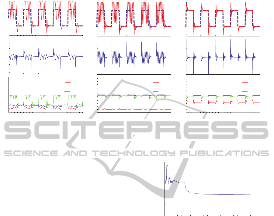
Figure 2: Example of the adaptation process controlled by the quantum neural self-tuning controller (top: plant output where
the dotted line indicates the desired plant output y
d
(k), and the rigid line indicates the plant output y(k); middle: control input
from the PID controller; bottom: output from the quantum neural network where the red line indicates K
P
(k), the blue line
indicates K
I
(k) and the green line indicates K
D
(k)).
[
∆ε(k) ε(k) ∆ε(k) − ∆ε(k− 1)
]. The initial val-
ues of θ
r
i, j
(0) and λ
r
j
(0) were randomly selected from
the interval [−π,π], and the initial value of δ
r
j
(0) was
set to 0.5. The learning factors were η = 10
−4
and
α = 0.9.
Figure 2 shows examples of the plant responses,
and Fig. 3 indicates the normalized cost function dur-
ing the adaptation process of the quantum neural self-
tuning controller. In Fig. 3, the horizontal axis repre-
sents the number of periods of the desired plant out-
put, and the vertical axis represents the normalized
cost function averaged within one period of the de-
sired plant output. The normalized cost function de-
creased as the training progressed. Although the over-
shoot and residual vibration are observed in the plant
output when the desired plant output changes rapidly,
the quantum neural self-tuning controller can achieve
the control task of making the non-linear plant follow
the desired plant output by tuning the gain parame-
ters with the output from the quantum neural network,
as shown in Fig. 2. These results indicate the fea-
sibility of the quantum neural self-tuning controller;
however, the control performance depends on the PID
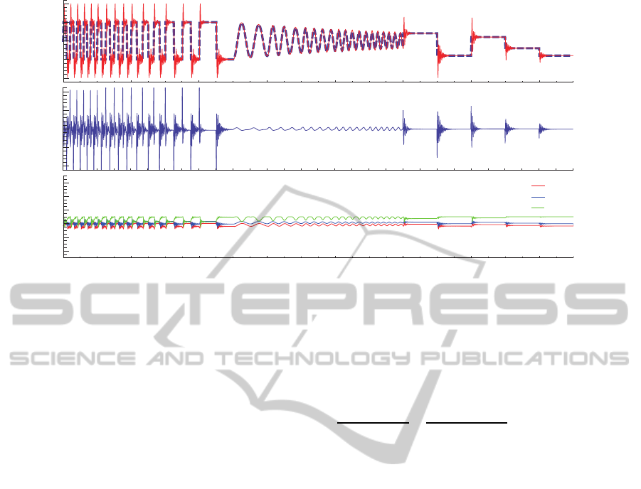
control law. To investigate the robustness of the quan-
tum neural self-tuning controller, other desired plant
outputs (e.g. a rectangular wave with various peri-
ods and amplitudes and a sinusoidal wave) are tested.
Here the initial values of the parameters θ
r
i, j
(0), λ
r
j
(0)
and δ
r
j
(0) are the trained parameters obtained after the
1000 periods shown in Fig. 3. Figure 4 shows the
response of the plant to the untrained desired plant
0 200 400 600 800 1000
10
-3
10
-2
10
-1
10
0
Period number
Normalized cost function
Figure 3: Relationship between the period number of the
desired plant output and the normalized cost function (con-
ventional controller: PID controller).
output. Using the learning capability of the quantum
neural self-tuning controller, the plant output tracks
the untrained desired plant output.
To demonstrate the extension of designing the
quantum neural self-tuning controller, a fuzzy logic
controller is considered as the conventionalcontroller.
Here the fuzzy logic controller is a velocity-type con-
troller, the output of which is the increment of the
control input ∆u(k) synthesized using the output er-
ror ε(k) and its difference ∆ε(k). Rutherford’s con-
trol rule is utilized as the fuzzy logic control rule
in which bell-shaped-type (Gaussian) membership
functions are used in the antecedent part, and sin-
gleton type membership functions are used in the
consequent part. The i-th fuzzy logic control rule
can be expressed by ’If ε(k) is A
i
and ∆ε(k) is B
i
then ∆u(k) is c
i
’, where A
i
and B
i
are fuzzy vari-
ables in the antecedent part, and c
i
is the position
ICINCO2013-10thInternationalConferenceonInformaticsinControl,AutomationandRobotics
110
0 400
Sampling number k
0
1
-1
0
1
Gain
800 1200200 600 1000 1400
0
1
-1
Output
Input
K (k)
P
K (k)
I
K (k)
D
Figure 4: Response of the plant controlled by the quantum neural self-tuning controller to untrained desired plant output (top:
plant output where the dotted line indicates the desired plant output y
d
(k), and the rigid line indicates the plant output y(k);
middle: control input; bottom: output from the quantum neural network where the red line indicates K
P
(k), the blue line
indicates K
I
(k) and the green line indicates K
D
(k)).
of the singleton type in the consequent part. The
fuzzy logic controller can be represented by ∆u(k) =
C
flc
(ε(k),∆ε(k),K
ε
,K
∆ε
,K
∆u
), where C
flc
(·) denotes
the fuzzy relation defined by the fuzzy logic con-
trol rule, and K
i
(i = ε,∆ε,∆u) represents the appro-
priate scale factors. In the antecedent and conse-
quent parts, the support of a fuzzy set has seven par-
titions which are normalized in the range [−6, 6] by
the scale factors. Using a simple fuzzy inference with
the settled values ε
o
(k) and ∆ε
o
(k), the output from
the fuzzy logic controller is calculated by ∆u
o
(k) =
∑
i
ζ
i
c
i
/
∑
i
ζ
i
, where ζ
i
is a fitness value in the an-
tecedent part given by ζ
i
= A
i
(ε
o
(k))B
i
(∆ε
o
(k)). In
the quantum neural self-tuning controller, the scale
factors in the antecedent part, K
ε
and K
∆ε
, are tuned
by the output from the quantum neural network. Be-
cause the fuzzy logic controller can be considered as
a non-linear PI controller by considering an analogy
to the PID controller, the input vector of the quantum
neural network x(k) can be defined as follows:
x(k) = [
y
d
(k+ d) y(k) · ·· y(k− n + 1)
u(k− 1) ·· · u(k− m − d + 1) δ
2
δ
3
∆ε(k)
δ
2
∆ε(k) δ
1
ε(k) det(e(k)e
T
(k) + D)
].
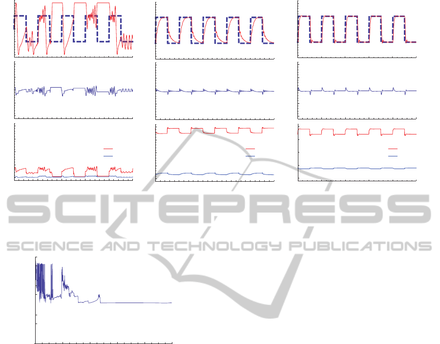
Figure 5 illustrates examples of the plant re-
sponses, and Fig. 6 shows the normalized cost func-
tion during the adaptation process of the quantum
neural self-tuning controller. Here the plant was
Eq. (12), and the quantum neural network was a
7–14–2 network topology in which the parameters
were the same as the case in which the conven-
tional controller was the PID controller, with the
exception of η = 10
−5
. Because the Jacobian of
the fuzzy logic controller is hard to calculate an-
alytically, it was approximated by ∂u(k)/∂u
n
(k) ≈
[
∆u(k)−∆u(k−1)
K
ε
(k)−K
ε
(k−1)
∆u(k)−∆u(k−1)
K
∆ε
(k)−K
∆ε
(k−1)
]. The scale factor
in the consequent part K
∆u
was 0.1. As shown in
Fig. 6, the normalized cost function decreased as
the training progressed and the quantum neural self-
tuning controller can make the plant output follow the
desired plant output by tuning the scale factors in the
fuzzy logic controller, as shown in Fig. 5. This re-
sult indicates the usefulness of applying the quantum
neural self-tuning controller to many types of conven-
tional controller.
4 CONCLUSIONS
This paper presented an adaptive-type self-tuning
controller based on a multi-layer quantum neural net-
work which uses qubit neurons as an information
processing unit, and investigated its characteristics
for control systems. We proposed a design of the
quantum-neural-network-based self-tuning controller
which conducts the training of the quantum neural
network as an online process. For a conventional con-
troller in which parameters are tuned by the quantum
neural network, a digital PID control law was uti-
lized. Computational experiments for the control of
a single-input single-output non-linear discrete-time
plant were conducted to evaluate the learning perfor-
mance and capability of the adaptive-type quantum
neural self-tuning controller. To investigate the use-
RemarksonanAdaptive-typeSelf-tuningControllerusingQuantumNeuralNetworkwithQubitNeurons
111
50000
50500
Sampling number k
Scale factor
30000
30500
Sampling number k
0
1
-1
Input
0
Scale factor
0
500
Sampling number k
0
1
-1
Input
2
0
Scale factor
0
1
-1
Output
0
1
-1
Output
0
1
-1
Output
0
1
-1
Input
K (k)
ε
K (k)
Δε
K (k)
ε
K (k)
Δε
K (k)
ε
K (k)
Δε
1
2
1
2
0
1
Figure 5: Example of the adaptation process controlled by the quantum neural self-tuning controller (top: plant output where
the dotted line indicates the desired plant output y
d
(k) and the rigid line indicates the plant output y(k); middle: control input
from the fuzzy logic controller; bottom: output from the quantum neural network where the red line indicates K
ε
(k) and the
blue line indicates K
∆ε
(k)).
0 200 400 600 800 1000
10
-3
10
-2
10
-1
10
0
Period number
Normalized cost function
Figure 6: Relationship between the period number of the
desired plant output and the normalized cost function (con-
ventional controller: fuzzy logic controller).
fulness of the quantum neural self-tuning controller,
the controller was also applied to tune the parameters
of a fuzzy logic controller. The results of the com-
putational experiments confirmed both the feasibility
and effectiveness of the adaptive-type quantum neural
self-tuning controller.
REFERENCES
Ezhov, A. A. and Ventura, D. (2000). Quantum neural net-
works. In Future Directions for Intelligent Systems
and Information Sciences, pages 213–234. Physica-
Verlang.
Hagan, M. T., Demuth, H. B., and Jesus, O. D. (2002). An
introduction to the use of neural networks in control
systems. International Journal of Robust and Nonlin-
ear Control, 12(11):959–985.
Kouda, N., Matsui, N., Nishimura, H., and Peper, F. (2005).
Qubit neural network and its learning efficiency. Neu-
ral Computing and Application, 14(2):114–121.
Manju, A. and Nigam, M. J. (2012). Applications of quan-
tum inspired computational intelligence: A survey. In
Artificial Intelligence Review, pages 1–78. Springer
Netherlands.
Meireles, M. R. G., Almeida, P. E. M., and Simoes, M. G.
(2003). A comprehensive review for industrial appli-
cability of artificial neural networks. IEEE Transac-
tions on Industrial Electronics, 50(3):585–601.
Sommer, G. (2001). Geometric Computing with Clifford
Algebra. Springer.
Takahashi, K., Kurokawa, M., and Hashimoto, M. (2011).
Controller application of a multi-layer quantum neu-
ral network trained by a conjugate gradient algorithm.
In Proceedings of the 37th Annual Conference of
the IEEE Industrial Electronics Society, pages 2278–
2283.
Yamada, T. (2011). Discussion of neural network con-
trollers from the point of view of inverse dynamics
and folding behaviour. In Proceedings of SICE An-
nual Conference 2011, pages 2210–2215.
Zhou, R., Qin, L., and Jiang, N. (2006). Quantum percep-
tron network. In Proceedings of the 16th International
Conference on Artificial Neural Networks, volume 1,
pages 651–657.
ICINCO2013-10thInternationalConferenceonInformaticsinControl,AutomationandRobotics
112
