
On Automated Recognition of Cloud Types Instructions
Nina Aprausheva
1
, Irina Gorlach
2
, Aleksandr Zhelnin
1
and Stanislav Sorokin
1
1
Computing Center: Russian Academy of Sciences,
Vavilov st. 40, 119333 Moscow, Russia
2
Hydrometeorological Research Center of Russian Federation,
11-13, B. Predtechensky per., 132242 Moscow, Russia
Abstract. Results of the recognition of multi-spectral satellite data by an auto-
mated classification procedure (ACP) are presented. The procedure is based on
the approximation of an unknown probability density of a given set of observa-
tions by a multi-dimensional Gaussian mixture. For a given number of mixture
components, optimal estimates for unknown parameters are found by the Day-
Shlezinger algorithm as such solution of simultaneous likelihood equations, that
maximizes the likelihood function. Optimal number of classes is determined by
the step-by-step testing of two composite statistical hypotheses. The classifica-
tion of a set of observations is performed by the Bayes rule. To reduce the cal-
culus number, a preliminary analysis of the structure of the investigated set is
carried out, which provides rough estimates of the number of classes and their
basic characteristics. Results of automatic classification of the main types of
clouds and underlying surface are described.
1 Introduction
The data on clouds and thermal characteristics of the Earth's atmosphere and surface
are widely used both in synoptical practice and in models employed in weather fore-
cast and analysis. Therefore, the development of automated methods for recognition
of various types of clouds is a topical problem. Data obtained from measurements by
high-resolution radiometers aboard geostationary satellites is one of the most promis-
ing information sources. The large amounts of information received from satellites
and the need for fast processing make it necessary to apply mathematical methods of
pattern recognition to such data most promising.
The first experiments on automated recognition of satellite images based on
previously acquired data on various types of clouds under different geographic
conditions and attempts to use them as reference data have shown that methods of
data processing need further refinement [1-3]. The approach based on studies of
multispectral data on radiative transfer in clouds with different properties and on the
threshold classification of clouds did not lead to the development of highly efficient
automated recognition techniques [4, 5]. Application of statistical automated
classification algorithms to this problem has a number of advantages and improves
the efficiency of recognition to 75-80% [6, 7]. For this reason, this approach was
chosen for deciphering the parts of images containing relatively small areas occupied
by frontal clouds. We tested the statistical algorithm of automated classification based
Aprausheva N., Gorlach I., Zhelnin A. and Sorokin S..
On Automated Recognition of Cloud Types Instructions.
DOI: 10.5220/0004395001140120
In Proceedings of the 4th International Workshop on Image Mining. Theory and Applications (IMTA-4-2013), pages 114-120
ISBN: 978-989-8565-50-1
Copyright
c
2013 SCITEPRESS (Science and Technology Publications, Lda.)

on the approximation of an unknown probability density function for a given set of
observations by a multidimensional Gaussian mixture with different vectors of mean
values and equal covariance matrices.
2 Recognition Algorithm
A sample of n p-dimensional observations (p≥1, n > p) is given,
X
(n)
= {X
l
, ..., X
n
}, X
j
= {X
jl
..., X
jp
}, j = 1,2, ..., n, (1)
where all the features have the numerical values. The unknown probability density of
a given sample f(X, Θ) can be approximated by a mixture of k normal distributions
f
i
(μ
i
, Σ) [8, 9].
,Θ
,
,Σ
,
(2)
,
,
|
|
∙
1/2
Σ
′
,
where
is the prior probability of the s
th
component of the mixture,
is the expec-
tation value vector of the s
th
mixture component, and Σ is the covariance matrix:
0,
1,1,
,…,
,
,…,
,
.
In this model, a class is the universe described by a unimodal probability density
f
s
(μ
s
, Σ) (s = 1, 2, ..., k). For a known value of k, the optimal estimate Θ
opt
for Θ is as
such a solution of the simultaneous of likelihood equations (SLE) that maximizes the
likelihood function
,,Θ
|
|
/
2
/
1
2
′
(3)
For k=1 the SLE has a unique solution [10]; for k≥2, the SLE has several solutions,
which are obtained by the Day-Shlezinger algorithm for various initial conditions
[11].
The Day-Shlezinger algorithm is difficult to apply, because the probability P
opt
of
the random choice of an optimal initial values Θ depends on the dimension p of the
sample space, the Mahalonobis distances ρ
st
between classes (s, t = 1, 2, ..., k), the
directions of the major axes of scattering ellipsoids, and the number of classes k [12,
13]. When the values of ρ
st
(s, t = 1, 2, ..., k) are small, then P
opt
may approach zero.
Therefore a preliminary analysis of the structure of the investigated set X
(n)
is is car-
ried out towards representative subsample X ' obtained from (1) by random choice
without replacement. Such analysis provides rough estimates for the number of clas-
ses k and their basic characteristics [14].
115

Introducing on the set X
(n)
the Euclid distance d, we calculate the distances d
mi
be-
tween all the different elements of the supsample X ', m <i, m = 1,2, ..., n
l
–1,
i = 2, 3, ..., n
l
, n
l
is the volume X ', n
l
≪ n. Arranging the set {d
mi
} in increasing or-
der, we construct the basic variational series (BVS) of the set X. An analysis of the
BVS provides the estimates of the low bound k
0
for the number of classes k and for
the maximal diameter d
max
of the classes. Then, we apply a cluster-analysis algorithm
[15] towards the subsample X ' to obtain rough estimates for the mixture parameters,
k
0
, π
0s
, μ
0s
, Σ
0
, s = 1,2, ..., k
0
, (4)
which are used as the first guesses in the Day-Shlezinger algorithm.
An optimal estimate k
opt
for the parameter k is determined by two methods. One is
based on consecutive testing of two composite hypotheses, H
k
and H
k+1
(k = k
0
– 1, k
0
,
k
0
+ 1, ..., t, t ≪ n). The hypothesis H
k
assumes that sample (1) contains k classes [16].
Of all values of k tested consecutively, the optimal value k
l
is the first one for which
the hypothesis H
k
is not rejected. If the hypothesis H
k
is true, then the statistic
λ
k,k+1
=–2ln[L(X
(n)
,k, Θ
opt
(k))/ L(X
(n)
,k+1,Θ
opt
(k+1))] (5)
converges to the χ
2
-distribution with degrees of freedom, c, c = p + 1, p is the dimen-
sion of the sample space; L(X
(n)
, k, Θ
opt
(k)) is a value of the likelihood function of the
set (1) for a fixed value of k and Θ = Θ
opt
.
In the second method, the optimal value k
2
is a number equal to the highest value k
for which the sequence of values of asymptotic likelihood functions {L
ac
(X
(n)
, k, Θ
opt
}
(k = k
0
, k
0
+ 1, k
m
, ..., l, l≪n) increases monotonically [16]:
,,Θ
|
Σ
|
/
2π
/
π
exp
1
2
μ
Σ
μ
′
∈
,
(6)
where n
s
is the number of elements in the class ω
s
. If the estimates k
1
and k
2
are dif-
ferent, then either may be taken as optimal; one may be also k
opt
= min(k
1
, k
2
).
Provided k = k
opt
and Θ = Θ
opt
, the classification of observations (1) carries out by
the Bayes rule [10]: an element X
j
belongs to the class
(s
0
∈ {1, 2, ..., k
opt
}) for
which the value of the posterior probability is maximal,
/
exp
′/2∙
exp
/2
,
(7)
argmax
1,2,…,
.
(8)
Instead of the true values of mixture parameters, the values of the corresponding
optimal estimates are substituted into formula (7).
116

3 Recognition of Meteorological Satellite Data
To test our algorithm for recognition of the types of cloudness and underlying surface
based on multispectral satellite data, we selected three regions observed from the
NOAA and METEOSAT satellites. The recognition results for two regions were pre-
sented in [17]. We discuss here the recognition results for the most complex region,
located in the North Atlantic and observed on December 9, 1991 from the
METEOSAT satellite.
The sample volume for this region was 100 30 pixels (each pixel corresponds to
a square with side ~10 km). Data in infrared and water-vapor emission bands were
used as features. Thus, each pixel was described by two weakly correlated features
(their correlation coefficient was 0.4):
,
,
1,…,3000.
(9)
A preliminary analysis of a subsample of volume n
1
= 450 was performed to obtain a
lower bound for the number k (k≥7) and the maximal diameter
d
max
= 30. The first guesses k
0
and Θ
0
were obtained by classifying this subsample by
MacQueen algorithm, where d
0
= d
max
/2 was used as a threshold value for intraclass
distances [15]; the corresponding estimate k
0
= 7. Varying the value of d
0
(d
0
= 16, 15,
14, 12, 10), according to MacQueen algorithm, we obtained different estimates for k
0
and Θ
0
(k
0
= 6, ...,10). For each of these values of k
0
, the estimates for the components
of Θ were refined by applying the Day-Shlezinger algorithm to subsamples of vol-
umes n
1
= 450 and n
2
= 750. An optimal value of k was determined from a set of val-
ues (k = 6, ..., 10) by the values of the statistic λ
k,k+1
(see (5)) for these subsamples
presented in Table 1. Setting the significance level at α = 0.02, we found that χ
.
(3)
= 9.8 by the table of χ
2
distribution with three degrees of freedom [18]. From the data
of Table 1 we have λ
6.7
> 9.8, λ
7.8
> 9.8, and λ
8.9
< 9.8 for the two subsamples. There-
fore, k
1
= 8.
Table 1. The values of the statistic λ
k,k+1
.
N
λ
6.7
λ
7.8
λ
8.9
λ
9.10
450
30 34 8
76
750
34 58
7 –50
Table 2. The values of logarithms of asymptotic likelihood function.
N
L
ac
(
6
)
L
ac
(
7
)
L
ac
(
8
)
L
ac
(
9
)
L
ac
(
10
)
450
–3169 –3150 –3126 –3116 –3175
750
–6375 –6344 –6314 –6317 –6379
Table 2 shows the values of logarithms of asymptotic likelihood function (6) for k
= 6, ..., 10 obtained for the same subsamples.
The second estimation method for k yields k
2
= 9 for the subsample of volume 450
and k
2
= 8 for the Table 1 subsample of volume 750. Therefore, k
opt
= 8 [19], and the
vector Θ
0
in (4) for k
0
= 8 was taken as the initial value of Θ in the Day-Shlezinger
algorithm. For k
opt
= 8, the estimate for the vector parameter Θ was refined by apply-
ing the Day- Shlezinger algorithm, so as to use this estimate in classifying the obser-
117
vation data by the Bayesian rule. Since the computer employed in this study had lim-
ited RAM resources, instead of inputting sample (9) as a whole, each of its three in-
dependent subsamples of volume n
i
=1100 (i=1, 2, 3), obtained by random sampling
without replacement, was processed separately. Note that some of the observation
data were left out of the subsamples.
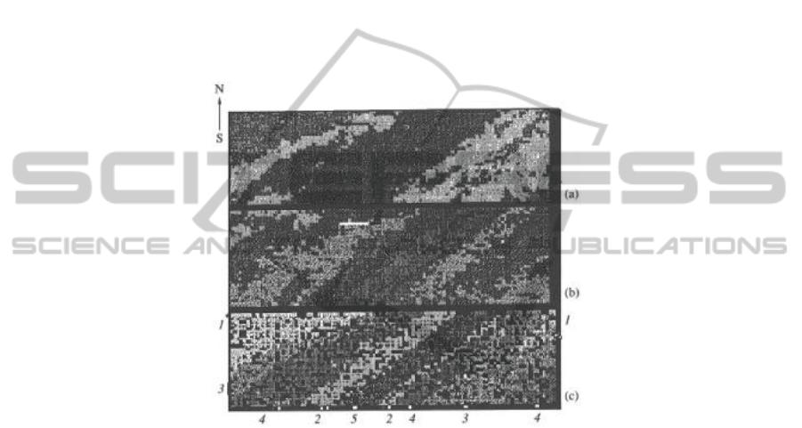
The figure shows the images of the region under investigation. Panel (a) contains
an infrared image obtained in the 10.5-12.5 μm band; the image obtained in the water-
vapor emission band (5.7-7.1 μm) is shown in panel (b); panel (c) contains the image
obtained as a result of algorithmic classification. The structure of an integral represen-
tation of clouds and sea surface observed from a satellite is easily seen here. Black
squares correspond to the observation data from (9) not included in each of the three
samples.
Fig. 1. The images of the region under investigation.
An analysis of synoptic data and isobaric maps shows that the selected region is
characterized by two distinct fronts with a band structure of cloud types, oriented
from southwest to northeast. The algorithm identified the image classes corresponding
to four basic cloud types: (1) heavy nimbostratus, (2) cirriform cloud, (3) stratiform
cloud, and (4) stratocumulus and (5) underlying sea surface. In addition, very small
classes of reference data points and flashes of reflected light were identified.
The estimates of the mean values of two indicators sorted by classes, obtained by
applying the Day-Shlezinger algorithm to one of the subsamples of volume n
i
= 1100,
are presented in Table 3 (in arbitrary units). The estimates of the variances
11
and
22
correlation coefficient ̃
12
) are equal for all of the eight classes:
11
= 44,
22
= 81,
21
= –14, ̃
12
= –0.2. Note that the value of the correlation coefficient ̃
12
had changed
drastically, from 0.4 before the classification to –0.2 after it.
The analysis of all results of automated recognition of satellite information for the
three selected regions suggests that successful recognition of cloud formations and
underlying surface can be performed by means of the above algorithm for any region
around the globe.
118

Table 3. The estimates of the mean values.
Class
number, s
Average A priori
probability, π
s
μ
s
1
μ
s
2
1 199 148 0.17
2 139 88 0.25
3 180 129 0.29
4 151 120 0.26
5 140 42 0.12
6 28 264 0.004
7 36 142 0.002
8 117 174 0.005
References
1. Solov'eva, I. S., Sonechkin, D. M., and Kharitonov, V. F.: Computerized Processing and
Analysis of Television Images of Clouds. In Tr. Gidrometeorol. Nauchno-Issled. Tsentra
(1971) no. 73, 64-74
2. Bakst, L. A. and Fedorova, N. N.: A Study of Clouds for Synoptic Analysis Based on Mul-
tispectral AVHRR Data from a NOAA Satellite. In Issl. Zemli iz Kosmosa (1994) no. 4, 3-
8
3. Tokuno, M. and Tsuchija, K.: Classification of Cloud Types Based on Data of Multiple
Satellite Sensors. In Adv. Space Res. (1994) Vol. 14, no. 3, 199-206
4. Peak, J. E. and Tag, P. M.: Segmentation of Satellite Imagery Using Hierarchical Thresh-
olding and Neural Networks. In J. Appl. Meteorol. (1994) Vol. 33, no. 5, 605-616
5. Strabala, K. I., Ackerman, S. A., and Menzel, W.P.: Cloud Properties Inferred from 8-12
μm Data. In J. Appl. Meteorol. (1994) Vol. 33, no. 2, 212-219
6. Bakst, L. and Fedorova, N.: On Some Methods of Synoptic Analysis Based on the Study of
the Multispectral Satellite Data Variation. In Proc. 9th Meteorological Satellite Data Users'
Conj.. Locarno, Switzerland, Darmstadt: EUMETSAT (1992) 25-32
7. Bankertt, R. L.: Cloud Classification of AVHRR Imagery in Maritime Regions Using a
Probabilistic Neural Network. In J. Appl. Meteorol. (1994) Vol. 33, no. 8, 1023-1039
8. Voloshin, G.Ya., Burlakov, I.A., and Kosenkova, S.T.: Statisticheskie metody resheniya
zadach raspoznavaniya, osnovannye na approksimatsionnom podkhode (Statistical Methods
for Recognition Problems Based on the Approximation Approach). Vladivostok, ch. 1
(1992)
9. Careira-Perpiñán, M. A., Williams, C.: On the number of modes of a Gaussian mixture.
Inform. In Res. Report EDI-INF-RR-0159. School of Inf. Univ. of Edinburg (2003)
10. Anderson, T. W.: An Introduction to Multivariate Statistical Analysis. Wiley, New York
(1958). Translated under the title Vvedenie v mnogomernyi statisticheskii analiz. Fizmat-
giz, Moscow (1963)
11. Day, N. E.: Estimating the Components of a Mixture of Normal Distributions. In Bio-
metrika (1969) Vol. 56, no. 3, 463-474.
12. Aprausheva, N. N.: Analysis of a Splitting Algorithm for the Mixture of Normally Distrib-
uted Classes, In Aivazyan. S.A. (ed.): Mnogomernyi statisticheskii analiz v sotsial'no-
ekonomicheskikh issledovaniyakh (Multidimensional Analysis in Social and Economic
Studies), Nauka, Moscow (1974) 135-150
13. Aprausheva, N. N.: Transformation of Features in the Statistical Solution of an Automated
Classification Problem. In Izv. Akad. Nauk SSSR, Ser: Tekhn. Kibern. (1985) no. 2, 167-
174
119

14. Aprausheva, N. N.: Novyi podkhod k obnaruzheniyu klasterov (A New Approach in Clus-
ter Detection). Vychisl. Tsentr Ross. Akad. Nauk, Moscow (1993)
15. Duran, B. S. and Odell, P. L.: Cluster Analysis. A Survey, Springer., Berlin (1974). Trans-
lated under the title Klasternyi analiz, Statistika, Moscow (1975)
16. Aprausheva, N. N.:(1981) Determination of the Number of Classes in Classification Prob-
lems. In Izv. Akad. Nauk SSSR. Ser: Tekhn. Kibern. (1981) no. 3, 71-77, no. 5, 153-160.
17. Aprausheva, N. N., Bakst, L. A., Gorlach, I. A., et al.: On the Recognition of Types of
Frontal Clouds Based on Satellite Data. Vychisl. Tsentr Ross. Akad. Nauk, Moscow (1996)
18. Cramér, H.: Mathematical Methods of Statistics. Princeton Univ. Press, Princeton New
Jersey (1946). Translated under the title Matematicheskie metody statistiki. Mir, Moscow
(1976)
19. Wilkes, S. S.: Mathematical Statistics. Wiley, New York: (1962). Translated under the title
Matematicheskaya statistika. Nauka, Moscow (1973)
120
