Model-less 3D Head Pose Estimation using Self-optimized Local
Discriminant Embedding
∗
F. Dornaika
1,2
, A. Bosaghzadeh
1
and A. Assoum
3
1
University of the Basque Country EHU/UPV, San Sebastian, Spain
2
IKERBASQUE, Basque Foundation for Science, Bilbao, Spain
3
LaMA Laboratory, Lebanese University, Tripoli, Lebanon
Keywords:
3D Head Pose Estimation, Local Discriminant Embedding.
Abstract:
In this paper, we propose a self-optimized Local Discriminant Embedding and apply it to the problem of
model-less 3D head pose estimation. Recently, Local Discriminant Embedding (LDE) method was proposed
in order to tackle some limitations of the global Linear Discriminant Analysis (LDA) method. In order to
better characterize the discriminant property of the data, LDE builds two adjacency graphs: the within-class
adjacency graph and the between-class adjacency graph. However, it is very difficult to set in advance these
two graphs. Our proposed self-optimized LDE has two important characteristics: (i) while all graph-based
manifold learning techniques (supervised and unsupervised) are depending on several parameters that require
manual tuning, ours is parameter-free, and (ii) it adaptively estimates the local neighborhood surrounding
each sample based on the data similarity. The resulting self-optimized LDE approach has been applied to the
problem of model-less coarse 3D head pose estimation (person independent 3D pose estimation). It was tested
on two large databases: FacePix and Pointing’04. It was conveniently compared with other linear techniques.
The experimental results confirm that our method outperforms, in general, the existing ones.
1 INTRODUCTION
Linear Dimensionality Reduction (LDR) techniques
have been increasingly important in pattern recogni-
tion (Yan et al., 2007) since they permit a relatively
simple mapping of data onto a lower-dimensional
subspace, leading to simple and computationally ef-
ficient classification strategies. Many dimensional-
ity reduction techniques can be derived from a graph
whose nodes represent the data samples and whose
edges quantify the similarity among pairs of samples
(Yan et al., 2007). LPP is a typical graph-based LDR
method that has been successfully applied in many
practical problems. LPP is essentially a linearized
version of Laplacian Eigenmaps (Belkin and Niyogi,
2003). In (Wang et al., 2009), the authors proposed
a linear discriminant method called Average Neigh-
bors Margin Maximization (ANMM). It associates to
every sample a margin that is set to the difference be-
tween the average distance to heterogeneous neigh-
bors and the average distance to the homogeneous
neighbors. The linear transform is then derived by
∗
This work was partially supported by the Spanish Gov-
ernment under the project TIN2010-18856 and by the Na-
tional Council for Scientific Research, Lebanon (LCNRS)
under the project 03-10-11
maximizing the sum of the margins in the embedded
space.
In (Chen et al., 2005), the authors proposed a
method called Local Discriminant Embedding (LDE).
This embedding method computes a linear mapping
that simultaneously maximizes the local margin be-
tween heterogeneous samples and pushes the homo-
geneous samples closer to each other. It has been
shown that it is very difficult to set in advance the
best neighborhood sizes for the within- and between-
class graphs used by (Chen et al., 2005). Usually, the
most popular adjacency graph construction manner is
based on the K nearest neighbor and ε-neighborhood
criteria. Once an adjacency graph is constructed,
the edge weights are assigned by various strategies
such as 0-1 weights and heat kernel function. Unfor-
tunately, such adjacency graphs are artificially con-
structed in advance, and thus they do not necessarily
uncover the intrinsic local geometric structure of the
samples. This stems from the fact that is very difficult
to set in advance the best neighborhood sizes for the
within- and between-class graphs.
In this paper, we introduce a self-optimized LDE
that constructs the within- and between-class graphs
without any predefined neighborhood size. We adap-
tively estimate the local neighborhood surrounding
347
Dornaika F., Bosgahzadeh A. and Assoum A..
Model-less 3D Head Pose Estimation using Self-optimized Local Discriminant Embedding.
DOI: 10.5220/0004347503470352
In Proceedings of the International Conference on Computer Vision Theory and Applications (VISAPP-2013), pages 347-352
ISBN: 978-989-8565-48-8
Copyright
c
 2013 SCITEPRESS (Science and Technology Publications, Lda.)

each sample based on data density and similarity.
This makes the proposed algorithm parameter-free
and adapted to each data set without user intervention.
Besides, we apply the proposed method to the prob-
lem of coarse 3D head pose estimation from 2D im-
age snapshots. Manifold learning paradigms becomes
more and more used for solving such problems (e.g.,
(Yan et al., 2009)).
The remainder of the paper is organized as fol-
lows. Section 2 describes the proposed self-optimized
Local Discriminant Embedding in which the recon-
struction of adjacency graphs is based on samples.
Section 3 presents the application which deals with
coarse 3D head pose estimation from images. It also
presents some experimental results obtained with two
databases: FacePix and Pointing’04. Section 4 con-
cludes the paper. Throughout the text, capital bold
letters denote matrices and small bold letters denote
vectors.
2 PROPOSED PARAMETERLESS
LOCAL DISCRIMINANT
EMBEDDING
2.1 Two Parameter-free Adjacency
Graphs
We assume that we have a set of N labeled sam-
ples {x
i
}
N
i=1
⊂ R
D
. In order to discover both geo-
metrical and discriminant structure of the data mani-
fold, we build two adjacency graphs: the within-class
graph G
w
(intrinsic graph) and between-class graph
G
b
(penalty graph). Let l(x
i
) be the class label of
x
i
. For each data sample x
i
, we compute two sub-
sets, N
b
(x
i
) and N
w
(x
i
). N
w
(x
i
) contains the neigh-
bors sharing the same label with x
i
, while N
b
(x
i
) con-
tains the neighbors having different labels. Instead of
using a fixed size for the neighbors, each sample x
i
will have its own adaptive set of neighbors. The set is
computed in two consecutive steps. First, the average
similarity of the sample x
i
is derived from all its simi-
larities with the rest of the data set (Eq. (1)). Second,
the sets of neighbors N
w
(x
i
) and N
b
(x
i
) are computed
using Eqs. (2) and (3), respectively.
AS(x
i
) =
1
N
N
∑
k=1
sim(x
i
,x
k
) (1)
sim(x
i
,x
k
) is a real value that encodes the similarity
between x
i
and x
k
. It belongs to the interval [0,1].
Simple choices for this function are the Kernel heat
and the cosine. A high value for AS(x
i
) means that
the sample has a lot of similar (close) samples. A
very low value means that this sample has very few
similar (close) samples.
N
w
(x
i
) = {x
j
| l(x
j
) = l(x
i
),sim(x
i
,x
j
) > AS(x
i
)}
(2)
N
b
(x
i
) = {x
j
| l(x
j
) 6= l(x
i
),sim(x
i
,x
j
) > AS(x
i
)}
(3)
Equation (2) means that the set of within-class
neighbors of the sample x
i
, N
w
(x
i
), is all data samples
that have the same label of x
i
and that have a similarity
higher than the average similarity associated with x
i
.
There is a similar interpretation for the set of between-
class neighbors N
b
(x
i
). From Equations (2) and (3) it
is clear that the neighborhood size is not the same for
every data sample. This mechanism adapts the set of
neighbors according to the local density and similar-
ity between data samples in the original space.
Since the concepts of similarity and closeness of
samples are tightly related, one can conclude, at first
glance, that our introduced strategy is equivalent to
the use of an ε-ball neighborhood. It is worth noting
that there are two main differences: (i) the use of an
ε-ball neighborhood requires a user-defined value for
the ball radius ε, and (ii) the ball radius is constant for
all data samples, whereas in our strategy the threshold
(1) depends on the local sample.
Each of the graphs mentioned before, G
w
and G
b
,
is characterized by its corresponding affinity (weight)
matrix W
w
and W
b
, respectively. The matrices are
defined by the following formulas:
W
w,ij
=

sim(x
i
,x
j
) i f x
j
∈ N
w
(x
i
) or x
i
∈ N
w
(x
j
)
0, otherwise
W
b,ij
=

1 if x
j
∈ N
b
(x
i
) or x
i
∈ N
b
(x
j
)
0, otherwise
2.2 Optimal Mapping
A linear embedding technique is described by a ma-
trix transform that maps the original samples x
i
into
low dimensional samples A
T
x
i
. The number of
columns of A defines the new dimension. We aim
to compute a linear transform, A, that simultaneously
maximizes the local margins between heterogenous
samples and pushes the homogeneous samples closer
to each other (after the transformation). Mathemati-
cally, this corresponds to:
min
A
1
2
∑
i, j
kA
T
(x
i
− x
j
)k
2
W
w,i j
(4)
max
A
1
2
∑
i, j
kA
T
(x
i
− x
j
)k
2
W
b,ij
(5)
VISAPP2013-InternationalConferenceonComputerVisionTheoryandApplications
348

Using simple matrix algebra, the abovecriteria be-
come respectively:
J
homo
=
1
2
∑
i, j
kA
T
(x
i
− x
j
)k
2
W
w,ij
(6)
= trace
n
A
T
X(D
w
− W
w
)X
T
A
o
(7)
= trace

A
T
XL
w
X
T
A

(8)
J
hete
=
1
2
∑
i, j
kA
T
(x
i
− x
j
)k
2
W
b,ij
(9)
= trace
n
A
T
X(D
b
− W
b
)X
T
A
o
(10)
= trace

A
T
XL
b
X
T
A

(11)
where X = (x
1
,x
2
,...,x
N
) is the data matrix, D
w
de-
notes the diagonal weight matrix, whose entries are
column (or row, since W
w
is symmetric) sums of W
w
,
and L
w
= D
w
− W
w
denotes the Laplacian matrix as-
sociated with the graph G
w
.
The two individualoptimization objectivesEq. (4)
and Eq. (5) can be fused into one criterion:
J =
J
hete
J
homo
=
trace

A
T
XL
b
X
T
A

trace

A
T
XL
w
X
T
A

=
trace

A
T
e
S
b
A

trace

A
T
e
S
w
A

(12)
where the symmetric matrix
e
S
b
= XL
b
X
T
denotes
the locality preserving between class scatter matrix,
and the symmetric matrix
e
S
w
= XL
w
X
T
denotes the
locality preserving within class scatter matrix. The
trace ratio optimization problem (12) can be replaced
by the simpler, yet inexact trace form:
max
A
trace


A
T
e
S
w
A

−1

A
T
e
S
b
A


(13)
The columns of the sought matrix A are given by the
generalized eigenvectors associated with the largest
eigenvalues of the following equation:
e
S
b
a = λ
e
S
w
a
Despite the fact that our proposed framework is
similar to LDE framework, it is worthy to note that
the proposed computation of the affinity matrices W
b
and W
w
is based on concept of adaptive adjacency
graphs.
In many real world problems such as face recogni-
tion, both matrices XL
b
X
T
and XL
w
X
T
can be singu-
lar. This stems from the fact that sometimes the num-
ber of images in the training set, N, is much smaller
than the number of pixels in each image, D. To over-
come the complication of singular matrices, original
data are first projected to a PCA subspace or a ran-
dom orthogonal space so that the resulting matrices
XL
b
X
T
and XL
w
X
T
are non-singular.
3 MODEL-LESS 3D HEAD POSE
ESTIMATION
Background. The majority of work in 3D head
pose estimation deals with tracking full rigid body
motion (6 degrees of freedom) for a limited range of
motion (typically +/-45 out-of-plane) and relatively
high resolution images. Besides, such systems typ-
ically require a 3D model (Dornaika and Ahlberg,
2004; Dornaika and Davoine, 2006) as well as its
initialization. There is a tradeoff between the com-
plexity of the initialization process, the speed of the
algorithm and the robustness and accuracy of pose
estimation. Although the model-based systems can
run in real-time, they rely on frame-to-frame estima-
tion and hence are sensitive to drift and require rel-
atively slow and non-jerky motion. These systems
require initialization and failure recovery. For situ-
ations in which the subject and camera are separated
by more than a few feet, full rigid body motion track-
ing of fine head pose is no longer practical. In this
case, model-less coarse pose estimation can be used
(Guo et al., 2008; Aghajanian and Prince, 2009). It
can be performed on a single image at any time with-
out any model given that some pose-classified ground
truth data are learned a priori (Fu and Huang, 2006;
Raytchev et al., 2004; Ma et al., 2006). Coarse 3D
pose estimation can play an important role in many
applications. For instance, it can be used in the do-
main of face recognition either by using hierarchical
models or by generating a frontal face image.
Databases. We evaluate the proposed methods with
experiments on two public face data sets for face
recognition and pose estimation.
1. The FacePix
2
database includes a set of face im-
ages with pose angle variations. It is composed
of 181 face images (representing yaw angles from
−90
◦
to +90
◦
at 1 degree increments) of 30 differ-
ent subjects, with a total of 5430 images. All the
face images are 128 pixels wide and 128 pixels
high. These images are normalized, such that the
eyes are centered on the 57th row of pixels from
the top, and the mouth is centered on the 87th row
of pixels. The upper part of Figure 1 provides ex-
amples extracted from the database, showing pose
angles ranging from −90
◦
to +90
◦
in steps of 10
◦
.
In our work, we downsample the set and only keep
10 poses in steps of 20
◦
.
2. Pointing’04
3
Head-Pose Image Database consists
of 15 sets of images for 15 subjects, wearing
2
htt p : //www. f acepix.org/
3
htt p : //www− prima.inrialpes. f r/Pointing04/
Model-less3DHeadPoseEstimationusingSelf-optimizedLocalDiscriminantEmbedding
349

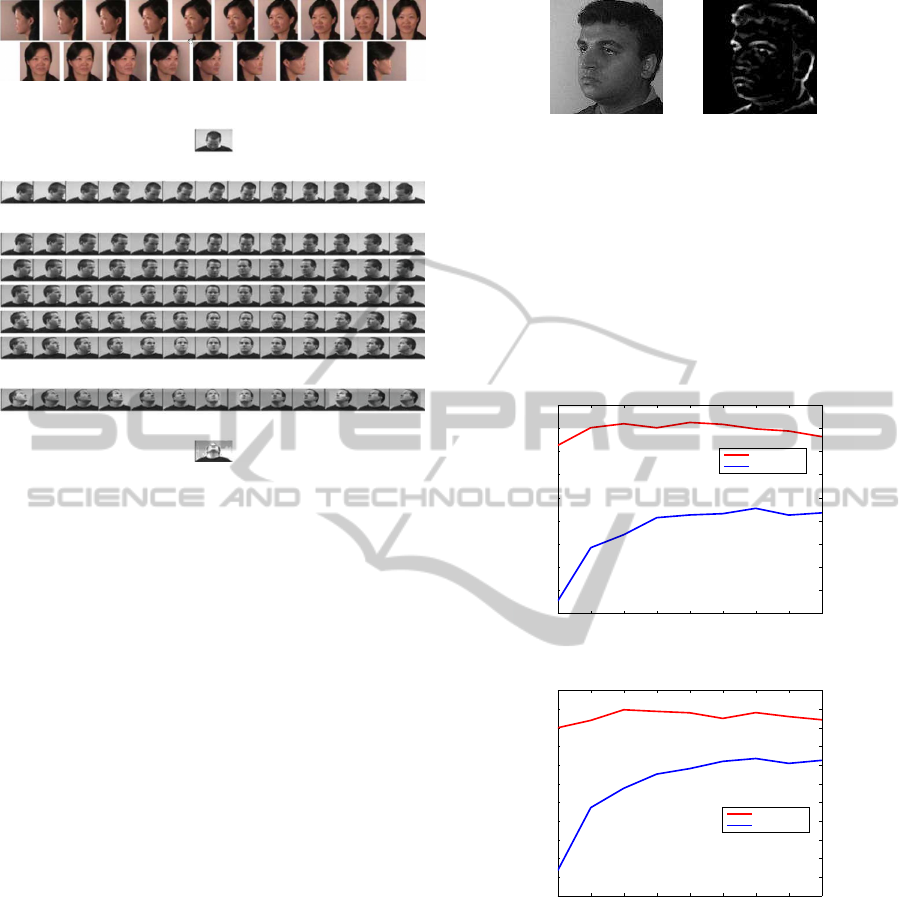
FacePix
Pointing’04
Figure 1: Some samples in FacePix and Pointing’04 data
sets.
glasses or not and having various skin colors.
Each set contains two series of 93 images of the
same person at different poses (lower part of Fig-
ure 1). In our work, we combine the two series
into one single data set so that we can carry out
tests on random splits. The pose or head orien-
tation is determined by the pan and tilt angles,
which vary from −90
◦
to 90
◦
in steps of 15
◦
.
Each pose has 30 images. The ground truth data
for this database are not as accurate as FacePix
data set. Indeed, the method used for generating
this data set belongs to directional suggestion cat-
egory which assumes that each subject’s head is
in the exact same physical location in 3D space
(Murphy-Chutorian and Trivedi, 2009). Further-
more, it assumes that persons have the ability
to accurately direct their head towards an ob-
ject. The effect of this limitation will be obvious
in the experimental results obtained with Point-
ing’04 data set.
Experimental Results. As mentioned earlier, the
problem of coarse 3D head pose estimation can be
cast into a classification problem. Estimating the pose
class of a test face image is carried out in the new
low dimensional space (obtained by the linear map-
ping) using the Nearest Neighbor classifier. We have
compared our method with four different methods,
namely: PCA, LPP, ANMM, and classic LDE. For
LPP, ANMM and classic LDE, five trials have been
(a) (b)
Figure 2: Image feature spaces used forthe experiments. (a)
Raw image. (b) Laplacian Of Gaussian (LOG) transformed
image.
performed in order to choose the optimal neighbor-
hood size. The final values correspond to those giving
the best recognition rate in test sets. For the experi-
ments, we used two representations: the raw images
and the Laplacian of Gaussian (LOG) transformed
images (See Figure 2).
10 20 30 40 50 60 70 80 90
36
38
40
42
44
46
48
50
52
54
Dimension
Recognition rate (%)
Pointing 04 Dataset: Pitch angle
Proposed LDE
Classic LDE
(a)
10 20 30 40 50 60 70 80 90
30
32
34
36
38
40
42
44
46
48
50
52
Dimension
Recognition rate (%)
Pointing 04 Dataset: Yaw angle
Proposed LDE
Classic LDE
(b)
Figure 3: Average classification accuracy for the clas-
sic LDE and the proposed method with Pointing’04 face
database. The number of training images per class is set to
20.
FacePix. For FacePix database, we have 10 differ-
ent classes, each with 30 subjects. For each class
(pose), l images are randomly selected for training
and the rest are used for testing. For each given l,
we average the results over several random splits. For
every split, the pre-stage of dimensionality reduction
(classical PCA) retained the top eigenvectors that cor-
respond to 95% of the total variability. In general, the
VISAPP2013-InternationalConferenceonComputerVisionTheoryandApplications
350

recognition rate varies with the dimension retained by
the embedding method. In all our experiments, we
recorded the best recognition rate for each algorithm.
Table 1 shows the correct classification rates for
different algorithms and for different number of train-
ing images per class, l. The algorithms used are:
PCA, LPP, ANMM, classic LDE with fixed neigh-
borhood size (fourth row), and the proposed self-
optimized LDE (fifth row). The number in parenthe-
sis depicts the dimension at which the rate is optimal
(highest one). As can be seen, our proposed approach
achieved 91.7% recognition rate when 25 face images
per pose/class were used for training, which is the
best out of the five algorithms (PCA, LPP, ANMM,
classic LDE, proposed method). Although the perfor-
mance of the proposed method is slightly better than
the competing methods, the latter ones need very te-
dious selection of the best neighborhood size param-
eters whereas the proposed method does not need any
parameter setting. We can also observe that proposed
approach with adaptive graphs can be superior to the
classical LDE adopting predefined graphs (See first
and second columns).
Table 2 shows the average error in the estimation
of the yaw angle for the raw images and the Lapla-
cian of Gaussian transformed images. This average
is computed over the all test images (those images
that are correctly classified has a zero error contribu-
tion). We can observe that the yaw angle estimation
obtained with the raw images is slightly better than
that obtained with the LOG transformed images.
In another experiment, we compared the classi-
fication performance of our proposed self-optimized
LDE method with the classic LDE. For the classic
LDE framework, several within-class graphs (param-
eterized by K
1
) and penalty graphs (parameterized by
K
2
) were built. Each pair (K
1
,K
2
) will give rise to
a given LDE transform. Table 3 summarizes the av-
erage correct classification rate of the yaw angle ob-
tained with the classic LDE and our proposed method
on the FacePix dataset. The classic LDE runs are pa-
rameterized by the pair of parameters (K
1
,K
2
). Every
rate was obtained as an average over 14 random splits.
The number of training images was set to 25. As can
be seen, the majority of the classic LDE runs gave a
recognition rate that is less than the one obtained with
our proposed self-optimized LDE.
Pointing04. Figure 3 depicts the correct classifica-
tion rate associated with the classic LDE and the pro-
posed self-optimized LDE when applied on Point-
ing’04 database. The number of training images per
class was 20. The classification is depicted as a func-
tion of the retained dimension of the embedded space.
Table 1: Best average classification accuracy (%) on
FacePix set over 14 random splits. Each column corre-
sponds to a fixed number of training images. The number
appearing in parenthesis corresponds to the optimal dimen-
sionality of the embedded subspace (at which the maximum
average recognition rate has been reported).
FacePix/ l 25 20 15
PCA 87.0% (30) 86.2% (30) 83.9% (30)
LPP 83.2% (20) 79.9% (20) 77.8 % (15)
ANMM 89.7% (15) 87.8% (10) 88.8% (10)
Classic LDE 90.2% (25) 88.5% (20) 88.2% (20)
Proposed LDE 91.7% (10) 89.6% (10) 88.1% (10)
Table 2: Average error (in degrees) in estimating the yaw
angle in FacePix database by varying the training size on
raw and LOG images.
FacePix / l 25 20 15
Raw images
Classic LDE 2.08
◦
2.30
◦
2.39
◦
Proposed Method 1.71
◦
1.85
◦
2.13
◦
LOG images
Classic LDE 2.28
◦
2.68
◦
2.91
◦
Proposed LDE 2.00
◦
2.54
◦
2.99
◦
Table 3: Classification accuracy (%) of the yaw angle
(Facepix dataset) using the proposed method as well as the
classic LDE. For the latter, we report the classification per-
formance obtained with several graphs configuration pa-
rameterized by K
1
and K
2
.
FacePix Yaw
Proposed LDE 91.7
Classic LDE K
2
=5 10 15 20 25
K
1
=5 90.7 89.7 89.7 89.4 89.1
K
1
=10 91.4 91.3 92.1 90.5 91.4
K
1
=15 91.5 91.4 90.7 90.7 91.0
K
1
=20 90.8 91.4 91.3 90.3 91.3
K
1
=25 90.7 91.4 90.7 90.4 90.8
As can be seen the proposed LDE outperformed the
classic LDE for all dimensions.
Table 4 shows the correct classification rates
for pitch and yaw angles obtained with PCA,
LPP, ANMM, classic LDE, and the proposed self-
optimized LDE method when applied on Pointing’04
data set. The number in parenthesis depicts the di-
mension at which the rate is optimal (highest one).
For these methods, the linear mapping was learned
using the 93 classes (poses). For a given test im-
age, the estimation of the pitch and yaw angle was
carried out in the embedded space using the Nearest
Neighbor classifier. On the other hand, the recogni-
tion rates were computed separately for the pitch and
yaw angles for all test images. The training set con-
tained 20 images per class. The test sets were formed
Model-less3DHeadPoseEstimationusingSelf-optimizedLocalDiscriminantEmbedding
351

solely by unseen subjects. The results are averaged
over ten random splits. As can be seen, our proposed
method achieved the best performance. We can also
observe that the proposed approach can be superior
to the classical LDE adopting predefined graphs. The
recognition rates were relatively low since the ground
truth data associated with Pointing’04 database were
not accurate.
Table 5 shows the average error in the estimation
of the pitch and yaw angles for the raw images and the
Laplacian of Gaussian transformed images. For both
kinds of images the errors were relatively small given
the fact that the resolution of the pitch and yaw angle
was 15
◦
. We can also observe that (i) for the pro-
posed method, the angle estimation (pitch and yaw)
obtained with the raw images is slightly better than
that obtained with the LOG transformed images, and
(ii) for the classic LDE, the angle estimation based on
the raw images was slightly worse than that based on
the LOG transformed images.
Table 4: Best average classification accuracy (%) on Point-
ing’04 data set for pitch and yaw angles (over 10 random
splits). The training sets contained 20 images.
Pointing’04 Pitch Yaw
PCA 46.5% (70) 47.8% (70)
LPP 45.3% (40) 44.9% (20)
ANMM 48.8% (70) 50.3% (70)
Classic LDE 45.1% (70) 44.7% (70)
Proposed LDE 52.5% (50) 49.9% (30)
Table 5: Average error in estimating the pitch and yaw an-
gles in Pointing’04 database on raw and LOG images (with
20 train image for each class).
Pointing’04 Pitch Yaw
Raw images
Classic LDE 14.12
◦
11.79
◦
Proposed LDE 11.64
◦
10.09
◦
LOG images
Classic LDE 13.86
◦
11.57
◦
Proposed LDE 13.02
◦
11.10
◦
4 CONCLUSIONS
We proposed a self-optimized Local Discriminant
Embedding method. We applied it to the problem
of model-less coarse 3D head pose estimation. We
used the proposed method as a generic (i.e. person-
independent) algorithm for head pose estimation. Un-
like many graph-based linear embedding techniques,
our proposed method does not need user-defined pa-
rameters. Experimental results carried out on the
problem demonstrate the advantage over some state-
of-art solutions and the classic LDE.
REFERENCES
Aghajanian, J. and Prince, S. (2009). Face pose estimation
in uncontrolled environments. In British Machine Vi-
sion Conference.
Belkin, M. and Niyogi, P. (2003). Laplacian eigenmaps
for dimensionality reduction and data representation.
Neural Computation, 15(6):1373–1396.
Chen, H., Chang, H., and Liu, T. (2005). Local discriminant
embedding and its variants. In IEEE International
Conference on Computer Vision and Pattern Recog-
nition.
Dornaika, F. and Ahlberg, J. (2004). Face and facial fea-
ture tracking using deformable models. International
Journal of Image and Graphics, 4(3):499–532.
Dornaika, F. and Davoine, F. (2006). On appearance
based face and facial action tracking. IEEE Transac-
tions on Circuits and Systems for Video Technology,
16(9):1107–1124.
Fu, Y. and Huang, T. (2006). Graph embedded analysis for
head pose estimation. In IEEE International Confer-
ence on Automatic Face and Gesture Recognition.
Guo, G., Fu, Y., Dyer, C., and Huang, T. (2008). Head
pose estimation: Classification or regression? In IEEE
International Conference on Pattern Recognition.
Ma, B., Zhang, W., Shan, S., Chen, X., and Gao, W. (2006).
Robust head pose estimation using lgbp. In Int. Con.
on Patt. Recog. ICPR’06.
Murphy-Chutorian, E. and Trivedi, M. (2009). Head
pose estimation in computer vision: a survey. IEEE
Trans. on Pattern Analysis and Machine Intelligence,
31(4):607–626.
Raytchev, B., Yoda, I., and Sakaue, K. (2004). Head pose
estimation by nonlinear manifold learning. In IEEE
International Conference on Pattern Recognition.
Wang, F., Wang, X., Zhang, D., Zhang, C., and Li, T.
(2009). Marginface: A novel face recognition method
by average neighborhood margin maximization. Pat-
tern Recognition, 42:2863–2875.
Yan, S., Wang, H., Fu, Y., Yan, J., Tang, X., and Huang,
T. (2009). Synchronized submanifold embedding
for person-independent pose estimation and beyond.
IEEE Trans. on Image Processing, 18(1):202–210.
Yan, S., Xu, D., Zhang, B., Zhang, H., Yang, Q., and Lin,
S. (2007). Graph embedding and extension: a gen-
eral framework for dimensionality reduction. IEEE
Trans. on Pattern Analysis and Machine Intelligence,
29(1):40–51.
VISAPP2013-InternationalConferenceonComputerVisionTheoryandApplications
352